Preprocessing

In this notebook, we cover functionality and recommendations for preprocessing data for modelling with Hidden Markov Models (HMM). Importantly, we assume that general preprocessing of fMRI, EEG/MEG, or physiological recordings has been performed using dedicated tools for each data modality, the GLHMM toolbox does not cover this. The tools provided in this toolbox only perform data wrangling to make your clean data ready for analysis. Once your data is ready for analysis, you can move on to the Gaussian HMM (suitable for fMRI data), the Gaussian-Linear HMM (for two sets of timeseries), or the time-delay embedded HMM (suitable for EEG/MEG data).

Note: Due to rendering issues when viewing this notebook through github, internal links, like the table of contents, may not work correctly. To ensure that the notebook renders correctly, you can view it through this link.

Authors: Christine Ahrends christine.ahrends@cfin.au.dk

Outline

0. Preface: Acquiring and preparing data for HMM-style analyses

1. Preparation

   • Load data

2. General syntax

   • Two sets of timeseries

3. Standardisation

4. Dimensionality reduction

   • Backtransforms

Preface: Acquiring and preparing data for HMM-style analyses

When preprocessing data for HMM-style analyses, it is important to keep in mind that between-subject noise and temporal noise may affect results more than in traditional task-based or temporal averaging analyses. For instance, poor registration in fMRI can lead to poor correspondence between parcels, which may drive the estimation to focus on artefactual between-subject differences, i.e. using states to cluster entire timeseries of subjects (Ahrends et al., Neuroimage 2022). Similarly, some parcellations and timecourse extraction methods may be better suited to capture temporal variance and less susceptible to between-subject noise than others (see Ahrends & Vidaurre in Filippi: fMRI Techniques & Protocols, 2025 for a detailed explanation). Compared to task-based analyses, where we would average out temporal noise over multiple trials, HMM-style dynamic analyses aim to find structure in temporal patterns in a data-driven way. In data that are heavily affected by temporal noise, such as motion or physiological artefacts like cardiac and respiratory activity, these patterns may dominate the more subtle patterns related to neural activity. Temporal preprocessing, e.g. using ICA clean-up (Hyvärinen, IEEE 1999, Ablin et al., IEEE 2018, Beckmann & Smith, IEEE 2004), can greatly reduce the influence of temporal artefacts on the estimation of dynamic neural patterns. Additionally, post-hoc correlation with head motion parameters and/or physiological recordings can be a good sanity-check.

Preparation

If you dont have the GLHMM-package installed, run the following command in your terminal:

pip install glhmm

Import libraries

Let’s start by importing the required libraries and modules.

import numpy as np
import pandas as pd
import matplotlib.pyplot as plt
import seaborn as sb
from glhmm import glhmm, preproc

Load data

Example data for this tutorial are available for download from the OSF. This notebook will fetch the relevant data from the OSF project page using the osfclient package. If you prefer, you can also directly download the files from the OSF project page and skip the next two cells.

# checks if osfclient is installed and otherwise installs it using pip install
# skip this if you have manually downloaded the data
import sys
import pip

def install(package):
    pip.main(['install', package])

try:
    import osfclient
except ImportError:
    print('osfclient is not installed, installing it now')
    install('osfclient')

! osf -p 8qcyj fetch GLHMM/data.csv ./example_data/data.csv
! osf -p 8qcyj fetch GLHMM/dataX.csv ./example_data/dataX.csv
! osf -p 8qcyj fetch GLHMM/T.csv ./example_data/T.csv

100%|██████████████████████████████████| 18.2M/18.2M [00:01<00:00, 16.7Mbytes/s]
100%|████████████████████████████████████| 496k/496k [00:00<00:00, 9.67Mbytes/s]
100%|███████████████████████████████████████| 218/218 [00:00<00:00, 617kbytes/s]

Synthetic data for this example should now be in the glhmm/docs/notebooks/example_data folder. The files data.csv and dataX.csv contain two sets of synthetic timeseries. The data should have the shape ((no subjects/sessions * no timepoints), no features), meaning that all subjects and/or sessions have been concatenated along the first dimension. The second dimension is the number of features, e.g., the number of parcels or channels. The file T.csv specifies the indices in the concatenated timeseries corresponding to the beginning and end of individual subjects/sessions in the shape (no subjects, 2). In this case, we have generated timeseries for 20 subjects and 50 features as the first timeseries, and the same 20 subjects and 2 features as the second timeseries. Each subject has 1,000 timepoints. The timeseries has the shape (20000, 50) and the indices have the shape (20, 2).

Input data for the glhmm should be in numpy format. Other data types, such as .csv, can be converted to numpy using e.g. pandas, as shown below. Alternatively, the io module provides useful functions to load input data in the required format, e.g., from existing .mat-files. If you need to create indices from session lengths (as used in the HMM-MAR toolbox) you can use the auxiliary.make_indices_from_T function.

data = pd.read_csv('./example_data/data.csv', header=None).to_numpy()
dataX = pd.read_csv('./example_data/dataX.csv', header=None).to_numpy()
T_t = pd.read_csv('./example_data/T.csv', header=None).to_numpy()

General syntax

The function preprocess_data contains all preprocessing tools available within the toolbox. You can configure it to do either a single or a combination of preprocessing steps appropriate for your data and model variety. Some of the most important preprocessing steps are described below, but see the documentation for all options.

The general syntax for preprocessing is:

data_preprocessed, indices_preprocessed, log = preprocess_data(data, indices, preprocessing_steps)
hmm = glhmm.glhmm(K=6, preproclogY=log)

The three outputs will be the preprocessed data, the preprocessed indices (only relevant for embedding), and a log. The log keeps track of which preprocessing steps have been performed and passes them onto the HMM. This is important so that we can later relate the parameter estimates of the HMM back to the original data.

Two sets of timeseries

When working with two sets of timeseries, e.g. for fitting a GLHMM, you will need to preprocess them separately. In this case, we will save the logs for both timeseries and pass both onto the HMM as preproclogX and preproclogY for timeseries X and Y, respectively:

dataX_preprocessed, indices_preprocessed, logX = preprocess_data(dataX, indices, preprocessing_steps)
dataY_preprocessed, indices_preprocessed, logY = preprocess_data(dataY, indices, preprocessing_steps)
hmm = glhmm.glhmm(K=6, preproclogX=logX, preproclogY=logY)

Standardisation

Standardisation refers to the process of transforming the timeseries to have mean zero and standard deviation 1. This makes sure that the state estimates in the HMM are not driven by spurious differences between subjects or channels. The function preprocess_data standardises the data by default. If you do not want to standardise your data, e.g. because they are already standardised, you can set standardise=False.

data_standard,_,log = preproc.preprocess_data(data, T_t)

The log is a dict containing a summary of which preprocessing steps have and which ones have not been performed:

log

{'fs': 1,
 'dampen_extreme_peaks': None,
 'standardise': True,
 'filter': None,
 'detrend': False,
 'onpower': False,
 'onphase': False,
 'pca': None,
 'exact_pca': True,
 'ica': None,
 'ica_algorithm': 'parallel',
 'post_standardise': None,
 'downsample': None,
 'files': None,
 'output_dir': None,
 'file_name': None,
 'file_type': 'npy',
 'lags': None,
 'p': 50,
 'N': 20}

In this case, since we have not specified any additional preprocessing steps, you can see that only standardise is set to True.

Dimensionality reduction (PCA/ICA)

It may sometimes be necessary to reduce the dimensionality of your data. Along the temporal axis, data can simply be downsampled by setting downsampling to the new frequency. This will mainly be relevant for EEG/MEG data or other recordings with high temporal resolution. Dimensionality reduction along the spatial dimension can be a crucial step to make sure the model is fitted appropriately, since too many free parameters to estimate from too few observations may cause the estimation to fail (Ahrends et al., NeuroImage 2022). This can happen, for instance, when using a very fine-grained parcellation but only few subjects, sessions, and time points (i.e., high spatial resolution but low temporal resolution and small number of subjects, as is often the case for fMRI studies). Another case for dimensionality reduction is when using the time-delay embedded HMM (Vidaurre et al., Nature Communications 2018), since the embedding greatly increases the number of parameters we need to estimate. As a rule of thumb, the ratio of observations to free parameters per state should not be inferior to 200. Dimensionality reduction along the spatial axis is commonly done using principal component analysis (PCA), where we will get components ordered by the amount of variance they explain, but the toolbox also offers functionality for independent component analysis (ICA). In both cases, you need to specify the number of components.

Note: We do not recommend to do PCA simply default because it may affect the state estimation in unexpected ways (Vidaurre, Plos Comput Biol 2021).

As an example, we can reduce the first timeseries we loaded from 50 features (brain regions/channels) to 10 using PCA. To do this, we simply set pca to the number of components:

data_small, _, log = preproc.preprocess_data(data, T_t, pca=10)

Compare dimensionalities between the original data and the new, reduced version:

print(f"The original data have {data.shape[0]} timepoints and {data.shape[1]} channels.")
print(f"The PCA-reduced data have {data_small.shape[0]} timepoints and {data_small.shape[1]} channels.")

The original data have 20000 timepoints and 50 channels.
The PCA-reduced data have 20000 timepoints and 10 channels.

Backtransforms

In order to relate the state estimates back to the original data, e.g. to plot the state maps, we need to backtransform them. This is done by default when calling any of the get_mean, get_beta, get_covariance_matrix and get_inverse_covariance_matrix and their respective plural functions.

hmm_small = glhmm.glhmm(K=3, covtype='full', model_beta='no', preproclogY=log)
hmm_small.train(X=None, Y=data_small, indices=T_t)

Init repetition 1 free energy = 442581.571519425
Init repetition 2 free energy = 442360.116591365
Init repetition 3 free energy = 442933.42136236414
Init repetition 4 free energy = 442984.87710992835
Init repetition 5 free energy = 442618.9072210602
Best repetition: 2
Cycle 1 free energy = 442519.97714597813
Cycle 2 free energy = 442298.9413386183
Cycle 3, free energy = 442266.87611784216, relative change = 0.12668941336304454
Cycle 4, free energy = 442247.7780633684, relative change = 0.07016208243852186
Cycle 5, free energy = 442232.33528270357, relative change = 0.053687528265280164
Cycle 6, free energy = 442218.74287235836, relative change = 0.045122389898996716
Cycle 7, free energy = 442206.40632006625, relative change = 0.0393421558151434
Cycle 8, free energy = 442195.7203524647, relative change = 0.03295526204943537
Cycle 9, free energy = 442186.6792765602, relative change = 0.027126113708118255
Cycle 10, free energy = 442178.7145000656, relative change = 0.023339139486833627
Cycle 11, free energy = 442171.2878601918, relative change = 0.021298732644099105
Cycle 12, free energy = 442163.9668119666, relative change = 0.020564145266982418
Cycle 13, free energy = 442156.56593401695, relative change = 0.020365023714391712
Cycle 14, free energy = 442149.16602470574, relative change = 0.019956006944492954
Cycle 15, free energy = 442141.86979887506, relative change = 0.0192967047230925
Cycle 16, free energy = 442134.9934375651, relative change = 0.01786143454824043
Cycle 17, free energy = 442128.85885149817, relative change = 0.01568473311915909
Cycle 18, free energy = 442123.49347133463, relative change = 0.013532411311415539
Cycle 19, free energy = 442118.8243649833, relative change = 0.011639222192973515
Cycle 20, free energy = 442114.7945640534, relative change = 0.009945642062754221
Cycle 21, free energy = 442111.36659658974, relative change = 0.008389326875699044
Cycle 22, free energy = 442108.5078532315, relative change = 0.006947646904939729
Cycle 23, free energy = 442106.14788837027, relative change = 0.005702750150835713
Cycle 24, free energy = 442104.1897874315, relative change = 0.0047093806449684935
Cycle 25, free energy = 442102.54512230534, relative change = 0.003939959161959472
Cycle 26, free energy = 442101.14670006046, relative change = 0.0033388743786618162
Cycle 27, free energy = 442099.9464401585, relative change = 0.0028575527581736586
Cycle 28, free energy = 442098.90969912906, relative change = 0.0024621733103075997
Cycle 29, free energy = 442098.01001263334, relative change = 0.0021321245770583473
Cycle 30, free energy = 442097.2254973115, relative change = 0.0018557356885802634
Cycle 31, free energy = 442096.53698729025, relative change = 0.0016259913168994577
Cycle 32, free energy = 442095.92720503954, relative change = 0.0014379963109175094
Cycle 33, free energy = 442095.3804262111, relative change = 0.0012877603687789666
Cycle 34, free energy = 442094.882608512, relative change = 0.001171075267318933
Cycle 35, free energy = 442094.42217044, relative change = 0.0010819708344397075
Cycle 36, free energy = 442093.9914863542, relative change = 0.0010110295407576885
Cycle 37, free energy = 442093.5886891306, relative change = 0.0009446719701811429
Cycle 38, free energy = 442093.21845952264, relative change = 0.0008675385404497548
Cycle 39, free energy = 442092.8898938984, relative change = 0.0007693173295421824
Cycle 40, free energy = 442092.61128110724, relative change = 0.0006519303810970116
Cycle 41, free energy = 442092.3852544622, relative change = 0.0005286036745115217
Cycle 42, free energy = 442092.2079783112, relative change = 0.00041442012272790985
Cycle 43, free energy = 442092.0717470221, relative change = 0.0003183677734871725
Cycle 44, free energy = 442091.96798775817, relative change = 0.00024242299946265498
Cycle 45, free energy = 442091.88903027156, relative change = 0.00018444213634930424
Cycle 46, free energy = 442091.82870303467, relative change = 0.0001409026189027332
Cycle 47, free energy = 442091.78230119887, relative change = 0.00010836617107645964
Cycle 48, free energy = 442091.7463297561, relative change = 8.400012656425659e-05
Cycle 49, free energy = 442091.7182179846, relative change = 6.564199755858002e-05
Cycle 50, free energy = 442091.69607608014, relative change = 5.16994703011761e-05
Cycle 51, free energy = 442091.6785081669, relative change = 4.1017905899425384e-05
Cycle 52, free energy = 442091.66447533417, relative change = 3.2763057728859505e-05
Cycle 53, free energy = 442091.6531974432, relative change = 2.6330283505235578e-05
Cycle 54, free energy = 442091.6440832305, relative change = 2.1278330906985168e-05
Cycle 55, free energy = 442091.6366805016, relative change = 1.7282347918648483e-05
Cycle 56, free energy = 442091.6306404298, relative change = 1.410090125470187e-05
Cycle 57, free energy = 442091.62569176056, relative change = 1.1552824627789334e-05
Reached early convergence
Finished training in 8.38s : active states = 3

(array([[2.81809377e-01, 1.93727210e-01, 5.24463414e-01],
        [3.22802970e-01, 1.10206666e-01, 5.66990364e-01],
        [2.18000426e-01, 3.57710033e-02, 7.46228570e-01],
        ...,
        [1.03698502e-04, 2.18228623e-05, 9.99874479e-01],
        [1.88332755e-02, 2.52356740e-03, 9.78643157e-01],
        [1.20768613e-01, 1.16941143e-02, 8.67537273e-01]]),
 array([[[2.60026838e-01, 1.36058963e-03, 2.04219493e-02],
         [4.98023612e-02, 1.08499509e-01, 3.54253396e-02],
         [1.29737710e-02, 3.46567470e-04, 5.11143075e-01]],

        [[2.03854869e-01, 1.37836165e-03, 1.17569739e-01],
         [1.21927749e-02, 3.43252341e-02, 6.36886571e-02],
         [1.95278226e-03, 6.74075435e-05, 5.64970174e-01]],

        [[2.29996198e-02, 1.58803874e-04, 1.94842003e-01],
         [4.43800189e-04, 1.27584166e-03, 3.40513614e-02],
         [1.75552463e-04, 6.18813745e-06, 7.46046830e-01]],

        ...,

        [[5.41965773e-08, 2.23225988e-09, 1.04227123e-06],
         [1.58995718e-09, 2.72663609e-08, 2.76935982e-07],
         [1.03642716e-04, 2.17933637e-05, 9.99873159e-01]],

        [[9.17474412e-05, 2.40002381e-06, 9.55103740e-06],
         [1.70033920e-06, 1.85193618e-05, 1.60316130e-06],
         [1.87398277e-02, 2.50264801e-03, 9.78632003e-01]],

        [[1.82049895e-02, 3.20554190e-04, 3.07731814e-04],
         [2.97436921e-04, 2.18059374e-03, 4.55367373e-05],
         [1.02266186e-01, 9.19296640e-03, 8.67184004e-01]]]),
 array([442519.97714598, 442298.94133862, 442266.87611784, 442247.77806337,
        442232.3352827 , 442218.74287236, 442206.40632007, 442195.72035246,
        442186.67927656, 442178.71450007, 442171.28786019, 442163.96681197,
        442156.56593402, 442149.16602471, 442141.86979888, 442134.99343757,
        442128.8588515 , 442123.49347133, 442118.82436498, 442114.79456405,
        442111.36659659, 442108.50785323, 442106.14788837, 442104.18978743,
        442102.54512231, 442101.14670006, 442099.94644016, 442098.90969913,
        442098.01001263, 442097.22549731, 442096.53698729, 442095.92720504,
        442095.38042621, 442094.88260851, 442094.42217044, 442093.99148635,
        442093.58868913, 442093.21845952, 442092.8898939 , 442092.61128111,
        442092.38525446, 442092.20797831, 442092.07174702, 442091.96798776,
        442091.88903027, 442091.82870303, 442091.7823012 , 442091.74632976,
        442091.71821798, 442091.69607608, 442091.67850817, 442091.66447533,
        442091.65319744, 442091.64408323, 442091.6366805 , 442091.63064043,
        442091.62569176]))

print(f"The shape of the state mean parameters before backtransforming is {hmm_small.mean[0]['Mu'].shape}")
print(f"The shape of the state covariance parameters before backtransforming is {hmm_small.mean[0]['Sigma'].shape}")

The shape of the state mean parameters before backtransforming is (10,)
The shape of the state covariance parameters before backtransforming is (10, 10)

state_means_orig = hmm_small.get_means()
print(f"The shape of the state means after backtransforming is {state_means_orig.shape}")

Transforming state mean back into original space
Transforming state mean back into original space
Transforming state mean back into original space
The shape of the state means after backtransforming is (50, 3)

state_covs_orig = hmm_small.get_covariance_matrices()
print(f"The shape of the state covariances after backtransforming is {state_covs_orig.shape}")

Transforming covariance matrix back into original space
Transforming covariance matrix back into original space
Transforming covariance matrix back into original space
The shape of the state covariances after backtransforming is (50, 50, 3)

If you do not want to backtransform the state parameters, you can set orig_space=False.

state_means_small = hmm_small.get_means(orig_space=False)
print(f"The shape of the state means in PCA-space is {state_means_small.shape}")

The shape of the state means in PCA-space is (10, 3)

state_covs_small = hmm_small.get_covariance_matrices(orig_space=False)
print(f"The shape of the state covariances in PCA-space is {state_covs_small.shape}")

The shape of the state covariances in PCA-space is (10, 10, 3)

You can also access the PCA model directly if you want to inspect it:

pcamodel = log["pcamodel"]
print(pcamodel.explained_variance_) # variance explained by each of the 10 first PCs
print(pcamodel.components_.shape) # weights (components x original features)

[9.6878944  7.23429978 4.0630088  3.06861996 2.64162666 2.2614071
 1.81425323 1.59480337 1.28083011 1.11603696]
(10, 50)

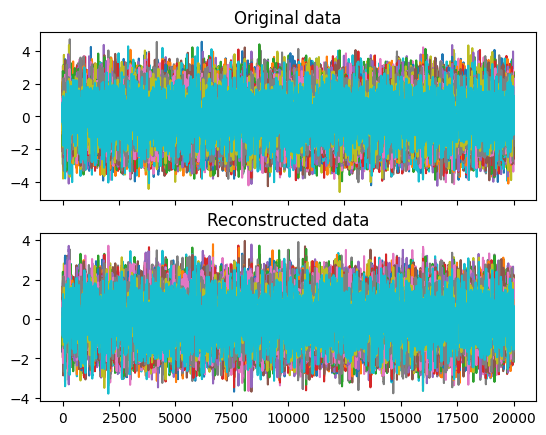
Using the components of the PCA model, you can manually backtransform. For instance, you can reconstruct the original data from the PCA-reduced version:

data_recon = data_small@pcamodel.components_

fig, (ax1, ax2) = plt.subplots(2,1, sharex=True)
ax1.plot(data_standard)
ax1.set_title("Original data")
ax2.plot(data_recon)
ax2.set_title("Reconstructed data")
plt.show()