Time-Delay Embedded and Multivariate Auto Regressive Hidden Markov Models
This notebook shows examples of training and inspecting a Time-Delay Embedded Hidden Markov Model (TDE-HMM) and a Multivariate Auto Regressive Hidden Markov Model (MAR-HMM).
The TDE-HMM and MAR-HMM are trained on Magnetoencephalogram (MEG) data. The TDE-HMM is trained on whole-brain data, while the MAR-HMM is trained on only two-channel data.
This notebook showcases also how to perform spectral analysis on the HMM states, including computing the states power spectra and the states cross-channel coherence.
Note: Due to rendering issues when viewing this notebook through github, internal links, like the table of contents, may not work correctly. To ensure that the notebook renders correctly, you can view it through this link.
Authors: Laura Masaracchia laurama@cfin.au.dk
Outline
TDE-HMM example
Load and preprocess data
Initialise and train a TDE-HMM
Spectral analysis
MAR-HMM example
Load data
Initialise and train a MAR-HMM
Relate states to behaviour
Spectral analysis
Background
The MAR-HMM was introduced in Vidaurre et al. (2016). Given a multichannel time series y, the MAR-HMM models estimates the probability of each time point of the data of belonging to state k by using a multivariate autoregressive model. This means that for each time point data yt, the MAR-HMM tries to find a linear combination of the previous P time points to predict yt. P is in this case a HMM parameter that has to be specified by the user, called “order”. The states here are the weights estimated in the prediction process.
The TDE-HMM was introduced in Vidaurre et al. (2018). This HMM models the autocovariance of the signal. Given a multichannel time series data y, the autocovariance is computed within a window of length 2L and resolution S around each time point yt. The window is specified by the user in the form (-L, -L+S, …-S, 0, S, …, L-S, L), which indicates the time points around t to be included in the window. Then, the data are restructured according to the lags embedding, and the HMM is run on the embedded data. Here, the states are the covariance matrices that best describe the signal.
The TDE-HMM is typically preferred for high-dimensional data, while the MAR-TDE can be more precise in detecting frequency and amplitude related states. Check Masaracchia et al. (2023) for a comparison between the MAR-HMM and TDE-HMM working mechanisms, biases and expected outcomes.
Preparation
If you dont have the GLHMM-package installed, then run the following command in your terminal:
!pip install git+https://github.com/vidaurre/glhmm
[1]:
!pip install git+https://github.com/vidaurre/glhmm
Collecting git+https://github.com/vidaurre/glhmm
  Cloning https://github.com/vidaurre/glhmm to /private/var/folders/43/6pvmtxkj1t31dy3ztfcww9cx1m_h0k/T/pip-req-build-f85z5cmt
  Running command git clone --filter=blob:none --quiet https://github.com/vidaurre/glhmm /private/var/folders/43/6pvmtxkj1t31dy3ztfcww9cx1m_h0k/T/pip-req-build-f85z5cmt
  Resolved https://github.com/vidaurre/glhmm to commit b4edad29e236e5688424a126243a925e54cbf212
  Installing build dependencies ... done
  Getting requirements to build wheel ... done
  Preparing metadata (pyproject.toml) ... done
Requirement already satisfied: scipy in /Users/au673157/anaconda3/lib/python3.11/site-packages (from glhmm==1.0.0) (1.10.1)
Requirement already satisfied: numpy in /Users/au673157/anaconda3/lib/python3.11/site-packages (from glhmm==1.0.0) (1.23.5)
Requirement already satisfied: scikit-learn in /Users/au673157/anaconda3/lib/python3.11/site-packages (from glhmm==1.0.0) (1.3.2)
Requirement already satisfied: matplotlib in /Users/au673157/anaconda3/lib/python3.11/site-packages (from glhmm==1.0.0) (3.7.1)
Requirement already satisfied: numba in /Users/au673157/anaconda3/lib/python3.11/site-packages (from glhmm==1.0.0) (0.58.0)
Requirement already satisfied: seaborn in /Users/au673157/anaconda3/lib/python3.11/site-packages (from glhmm==1.0.0) (0.13.2)
Requirement already satisfied: pandas in /Users/au673157/anaconda3/lib/python3.11/site-packages (from glhmm==1.0.0) (1.5.3)
Requirement already satisfied: igraph in /Users/au673157/.local/lib/python3.11/site-packages (from glhmm==1.0.0) (0.11.3)
Requirement already satisfied: tqdm in /Users/au673157/anaconda3/lib/python3.11/site-packages (from glhmm==1.0.0) (4.66.6)
Requirement already satisfied: scikit-image in /Users/au673157/anaconda3/lib/python3.11/site-packages (from glhmm==1.0.0) (0.20.0)
Requirement already satisfied: statsmodels in /Users/au673157/anaconda3/lib/python3.11/site-packages (from glhmm==1.0.0) (0.14.0)
Requirement already satisfied: h5py in /Users/au673157/anaconda3/lib/python3.11/site-packages (from glhmm==1.0.0) (3.7.0)
Requirement already satisfied: nibabel in /Users/au673157/anaconda3/lib/python3.11/site-packages (from glhmm==1.0.0) (5.1.0)
Requirement already satisfied: requests in /Users/au673157/anaconda3/lib/python3.11/site-packages (from glhmm==1.0.0) (2.31.0)
Requirement already satisfied: nilearn in /Users/au673157/anaconda3/lib/python3.11/site-packages (from glhmm==1.0.0) (0.10.4)
Requirement already satisfied: texttable>=1.6.2 in /Users/au673157/.local/lib/python3.11/site-packages (from igraph->glhmm==1.0.0) (1.7.0)
Requirement already satisfied: contourpy>=1.0.1 in /Users/au673157/anaconda3/lib/python3.11/site-packages (from matplotlib->glhmm==1.0.0) (1.0.5)
Requirement already satisfied: cycler>=0.10 in /Users/au673157/anaconda3/lib/python3.11/site-packages (from matplotlib->glhmm==1.0.0) (0.11.0)
Requirement already satisfied: fonttools>=4.22.0 in /Users/au673157/anaconda3/lib/python3.11/site-packages (from matplotlib->glhmm==1.0.0) (4.25.0)
Requirement already satisfied: kiwisolver>=1.0.1 in /Users/au673157/anaconda3/lib/python3.11/site-packages (from matplotlib->glhmm==1.0.0) (1.4.4)
Requirement already satisfied: packaging>=20.0 in /Users/au673157/anaconda3/lib/python3.11/site-packages (from matplotlib->glhmm==1.0.0) (23.0)
Requirement already satisfied: pillow>=6.2.0 in /Users/au673157/anaconda3/lib/python3.11/site-packages (from matplotlib->glhmm==1.0.0) (10.0.1)
Requirement already satisfied: pyparsing>=2.3.1 in /Users/au673157/anaconda3/lib/python3.11/site-packages (from matplotlib->glhmm==1.0.0) (3.0.9)
Requirement already satisfied: python-dateutil>=2.7 in /Users/au673157/anaconda3/lib/python3.11/site-packages (from matplotlib->glhmm==1.0.0) (2.8.2)
Requirement already satisfied: joblib>=1.0.0 in /Users/au673157/anaconda3/lib/python3.11/site-packages (from nilearn->glhmm==1.0.0) (1.2.0)
Requirement already satisfied: lxml in /Users/au673157/anaconda3/lib/python3.11/site-packages (from nilearn->glhmm==1.0.0) (4.9.2)
Requirement already satisfied: pytz>=2020.1 in /Users/au673157/anaconda3/lib/python3.11/site-packages (from pandas->glhmm==1.0.0) (2022.7)
Requirement already satisfied: charset-normalizer<4,>=2 in /Users/au673157/anaconda3/lib/python3.11/site-packages (from requests->glhmm==1.0.0) (2.0.4)
Requirement already satisfied: idna<4,>=2.5 in /Users/au673157/anaconda3/lib/python3.11/site-packages (from requests->glhmm==1.0.0) (3.4)
Requirement already satisfied: urllib3<3,>=1.21.1 in /Users/au673157/anaconda3/lib/python3.11/site-packages (from requests->glhmm==1.0.0) (1.26.16)
Requirement already satisfied: certifi>=2017.4.17 in /Users/au673157/anaconda3/lib/python3.11/site-packages (from requests->glhmm==1.0.0) (2023.11.17)
Requirement already satisfied: threadpoolctl>=2.0.0 in /Users/au673157/anaconda3/lib/python3.11/site-packages (from scikit-learn->glhmm==1.0.0) (2.2.0)
Requirement already satisfied: llvmlite<0.42,>=0.41.0dev0 in /Users/au673157/anaconda3/lib/python3.11/site-packages (from numba->glhmm==1.0.0) (0.41.1)
Requirement already satisfied: networkx>=2.8 in /Users/au673157/anaconda3/lib/python3.11/site-packages (from scikit-image->glhmm==1.0.0) (3.1)
Requirement already satisfied: imageio>=2.4.1 in /Users/au673157/anaconda3/lib/python3.11/site-packages (from scikit-image->glhmm==1.0.0) (2.31.1)
Requirement already satisfied: tifffile>=2019.7.26 in /Users/au673157/anaconda3/lib/python3.11/site-packages (from scikit-image->glhmm==1.0.0) (2021.7.2)
Requirement already satisfied: PyWavelets>=1.1.1 in /Users/au673157/anaconda3/lib/python3.11/site-packages (from scikit-image->glhmm==1.0.0) (1.4.1)
Requirement already satisfied: lazy_loader>=0.1 in /Users/au673157/anaconda3/lib/python3.11/site-packages (from scikit-image->glhmm==1.0.0) (0.3)
Requirement already satisfied: patsy>=0.5.2 in /Users/au673157/anaconda3/lib/python3.11/site-packages (from statsmodels->glhmm==1.0.0) (0.5.3)
Requirement already satisfied: six in /Users/au673157/anaconda3/lib/python3.11/site-packages (from patsy>=0.5.2->statsmodels->glhmm==1.0.0) (1.16.0)
Building wheels for collected packages: glhmm
  Building wheel for glhmm (pyproject.toml) ... done
  Created wheel for glhmm: filename=glhmm-1.0.0-py3-none-any.whl size=165139 sha256=229b438093e10392f4b29f59b6f95489b010cfa06deb224f9654a589cfb1a5ee
  Stored in directory: /private/var/folders/43/6pvmtxkj1t31dy3ztfcww9cx1m_h0k/T/pip-ephem-wheel-cache-ah4l0at5/wheels/73/39/44/d3ee0c50a18e95f840c3481c25961f199ad5b37fb8b0bed2f2
Successfully built glhmm
Installing collected packages: glhmm
  Attempting uninstall: glhmm
    Found existing installation: glhmm 0.2.11
    Uninstalling glhmm-0.2.11:
      Successfully uninstalled glhmm-0.2.11
Successfully installed glhmm-1.0.0

[notice] A new release of pip is available: 24.2 -> 25.1
[notice] To update, run: pip install --upgrade pip
We will then import the necessary libraries and modules for this notebook
[1]:
import numpy as np
import matplotlib.pyplot as plt
from glhmm import glhmm, preproc, utils, graphics, spectral, io, statistics, auxiliary
import pickle
import sys
import pip
/Users/au673157/anaconda3/lib/python3.11/site-packages/_distutils_hack/__init__.py:26: UserWarning: Setuptools is replacing distutils.
  warnings.warn("Setuptools is replacing distutils.")
TDE-HMM Example: Modelling whole-brain MEG data
For this example, we will use whole-brain MEG resting state data. The data was collected from 10 participants while resting in a dark room. Each participant completed two sessions, except for one participant with only one session.
Each session is stored as a 2D matrix with the shape of (No. of timepoints, No. of parcels):
Timepoints: The total number of recorded time points in the session. Parcels: Here regions according to a prespecified parcellation.
The data we will load are a subset of the data collected and used for the original TDE-HMM paper
Load and preprocess data
The next two cells will fetch the data from the OSF website and download them into the same folder as this notebook. If you prefer, you can also directly download the files from the OSF project page and skip the next two cells.
[2]:
# checks if osfclient is installed and otherwise installs it using pip install
# skip this if you have manually downloaded the data

def install(package):
    pip.main(['install', package])

try:
    import osfclient
except ImportError:
    print('osfclient is not installed, installing it now')
    install('osfclient')
[3]:
! osf -p 8qcyj fetch MEG_data/data_MEG_TDE.pkl ./example_data/data_MEG_TDE.pkl
100%|████████████████████████████████████| 127M/127M [00:03<00:00, 39.2Mbytes/s]
We will then load the data into the notebook
NOTE: this cell is compulsory to all!
[4]:
# Loading the data

with open("./example_data/data_MEG_TDE.pkl", "rb") as f:
    data_meg_tde = pickle.load(f)

# Display data information
print(f"Number of sessions in data_meg: {len(data_meg_tde)}")
Number of sessions in data_meg: 5
Prepare data
Once we have loaded the data we need to make them in the right format for the HMM, meaning concatenate all sessions and subjects along the time axis. We also need to create the indices that will tell the start and end timepoint of each session:
Concatenated brain activity (X_concat) The brain activity data (data_meg) contains recordings from multiple sessions. We concatenate all the sessions along the time dimension to form a single, continuous 2D matrix: [timepoints × sessions, features].
Create index matrix (idx_data) To track the start and end timepoints for each session, we generate an index matrix, idx_data, using the function get_indices_from_list. It will have a shape of: [No. of sessions, 2]. Each row specifies the start and end timepoints for a session.
Loading data and data formats are explained in more detail in the Standard Gaussian HMM tutorial.
[5]:
# concatenate data
X_concat = []
for j in range(len(data_meg_tde)):
    X_concat.extend(data_meg_tde[j])

X_concat = np.array(X_concat)

# Get the start and end indices for each session
idx_data = statistics.get_indices_from_list(data_meg_tde)
[6]:
# show the session indices
idx_data
[6]:
array([[     0,  75685],
       [ 75685, 151447],
       [151447, 226381],
       [226381, 301893],
       [301893, 377536]])
NOTE: It is important to standardise your timeseries and, if necessary, apply other kinds of preprocessing before fitting the model.
We always recommend to plot the data before doing any preprocessing, and understand what preprocessing steps are needed.
The data for this tutorial have already been preprocessed, so we will only standardise them.
[7]:
# Preprocess data
X_preproc = preproc.preprocess_data(X_concat, idx_data)[0]
[8]:
# visualize some data
# decide on a plotting range of the signal
plot_range = np.arange(200000,202000)

Fs = 250 # sampling frequency of the signal
n_regions = X_preproc.shape[1]

# plot each parcel separately
fig = plt.figure(figsize=(10,8))
for i in range(n_regions):
    plt.plot(X_preproc[plot_range,i]+i*5)

plt.xticks(np.arange(0,len(plot_range),Fs),np.arange(int(len(plot_range)/Fs)))
plt.xlabel('time [s]')
plt.yticks(np.arange(0,n_regions*5,5),np.arange(n_regions))
plt.ylabel('parcel')
plt.title('Example of Preprocessed Signal')
plt.show()

Initialise and train a TDE-HMM
We first initialise the glhmm object, which we here call TDE_hmm. By specifying the parameters of the glhmm object, we define which type of model we want to fit and how states should be defined.
In the case of the TDE-HMM, this is done with two steps: we will first embed the data within a window of lags, then we will run a default (i.e. Gaussian) HMM on the embedded data.
For the first step, we will use the build_data_tdeoption in the preprocessing module. This will create an embedded version of the data according to the lags we define. The lags will indicate the length and resolution of the window to use to embed the data. In this specific case, our window of lags will be of length 2L, where L=35, with resolution S=5. The lags window will go from -35 to +35 with step of 5: embedded_lags = np.arange(-L,L+1,S). We will then use PCA on the embedded
signal, using number of PC=number of parcels * 2, to follow the original TDE-HMM paper preprocessing and HMM settings.
We will then run a Gaussian HMM on the embedded data, to capture the autocovariance of the signal.
We model 10 states by setting the parameter K=10. We will also specify the covariance type as covtype='full' and no means modelling. So our states will be characterised only by functional connectivity (covariance).
[9]:
# Specify time lags
S=5
L = 35
lags = np.arange(-L, L + 1, S)

# Build the MEG data in TDE format
X_embedded, idx_tde, pca_model = preproc.build_data_tde(X_preproc,idx_data,lags=lags,pca=n_regions*2)
[10]:
# instantiate model
K=10
TDE_hmm = glhmm.glhmm(model_beta='no', model_mean='state', K=K, covtype='full')
[12]:
# train HMM
print('Training HMM-TDE')

stc_tde, xi_tde, fe_tde = TDE_hmm.train(X=None, Y=X_embedded, indices=idx_tde)
vpath_tde = TDE_hmm.decode(X=None, Y=X_embedded, viterbi=True)
Training HMM-TDE
Init repetition 1 free energy = 63945242.26363943
Init repetition 2 free energy = 63960406.542562775
Init repetition 3 free energy = 63882160.247551166
Init repetition 4 free energy = 63867329.00079531
Init repetition 5 free energy = 63908398.950842775
Best repetition: 4
Cycle 1 free energy = 63857362.42757152
Cycle 2 free energy = 63846845.332875386
Cycle 3, free energy = 63840872.80908218, relative change = 0.3621990282593063
Cycle 4, free energy = 63837111.15853057, relative change = 0.1857488804283497
Cycle 5, free energy = 63833926.50930166, relative change = 0.1358875377630957
Cycle 6, free energy = 63831474.15989289, relative change = 0.0947282158550761
Cycle 7, free energy = 63829495.784432106, relative change = 0.07099439465613099
Cycle 8, free energy = 63827637.402728, relative change = 0.06251909675062768
Cycle 9, free energy = 63825891.29173486, relative change = 0.0554829352903556
Cycle 10, free energy = 63824374.01168278, relative change = 0.045994328954685346
Cycle 11, free energy = 63823074.337182924, relative change = 0.03790454601364171
Cycle 12, free energy = 63821723.76017774, relative change = 0.037896394673299576
Cycle 13, free energy = 63820724.0211532, relative change = 0.027286640503072886
Cycle 14, free energy = 63819787.16050876, relative change = 0.02493290714002275
Cycle 15, free energy = 63819057.75872617, relative change = 0.019042111694845088
Cycle 16, free energy = 63818403.79401329, relative change = 0.01678613065068411
Cycle 17, free energy = 63817759.66814152, relative change = 0.01626467147847695
Cycle 18, free energy = 63817148.54815109, relative change = 0.015196742996158459
Cycle 19, free energy = 63816674.28241634, relative change = 0.01165611587695376
Cycle 20, free energy = 63816262.87029992, relative change = 0.010010134992562059
Cycle 21, free energy = 63815968.787892655, relative change = 0.0071045312648853895
Cycle 22, free energy = 63815681.040631816, relative change = 0.006903495348055411
Cycle 23, free energy = 63815389.71620584, relative change = 0.00694080550181527
Cycle 24, free energy = 63815052.6827992, relative change = 0.007965857711000298
Cycle 25, free energy = 63814775.99890221, relative change = 0.006496996945602436
Cycle 26, free energy = 63814579.0749586, relative change = 0.004602817020691603
Cycle 27, free energy = 63814378.82569455, relative change = 0.004658736245969561
Cycle 28, free energy = 63814228.10416342, relative change = 0.003494236589835568
Cycle 29, free energy = 63814051.12208444, relative change = 0.004086279021009162
Cycle 30, free energy = 63813834.46039891, relative change = 0.004977528232991238
Cycle 31, free energy = 63813722.80231103, relative change = 0.0025586399336136913
Cycle 32, free energy = 63813616.74623246, relative change = 0.0024243782547021075
Cycle 33, free energy = 63813490.2783988, relative change = 0.00288264505034032
Cycle 34, free energy = 63813392.75755326, relative change = 0.002217911699118092
Cycle 35, free energy = 63813327.38728433, relative change = 0.0014845057140788437
Cycle 36, free energy = 63813218.37548818, relative change = 0.0024694560424192435
Cycle 37, free energy = 63813098.43528346, relative change = 0.0027096562808133972
Cycle 38, free energy = 63812969.505615436, relative change = 0.0029042843395558626
Cycle 39, free energy = 63812877.571343176, relative change = 0.0020666420003150783
Cycle 40, free energy = 63812807.15909478, relative change = 0.0015803349593133459
Cycle 41, free energy = 63812729.217802264, relative change = 0.0017462623217067744
Cycle 42, free energy = 63812654.68963167, relative change = 0.001667008308345958
Cycle 43, free energy = 63812591.537828565, relative change = 0.0014105550161867429
Cycle 44, free energy = 63812502.20867358, relative change = 0.0019912777328705243
Cycle 45, free energy = 63812402.936475195, relative change = 0.0022080365227844937
Cycle 46, free energy = 63812306.26506688, relative change = 0.002145575720258484
Cycle 47, free energy = 63812251.722074844, relative change = 0.0012090919756748886
Cycle 48, free energy = 63812209.953423984, relative change = 0.0009250578544846764
Cycle 49, free energy = 63812151.46746594, relative change = 0.0012936234468506405
Cycle 50, free energy = 63812088.27729245, relative change = 0.0013957230140131652
Cycle 51, free energy = 63812038.54028973, relative change = 0.0010973684232707386
Cycle 52, free energy = 63811979.2842319, relative change = 0.0013056843018834003
Cycle 53, free energy = 63811903.453207515, relative change = 0.0016681200015377523
Cycle 54, free energy = 63811810.7580577, relative change = 0.002034945168989832
Cycle 55, free energy = 63811727.9279695, relative change = 0.0018150760700905966
Cycle 56, free energy = 63811650.12052952, relative change = 0.001702111422890948
Cycle 57, free energy = 63811577.29433968, relative change = 0.0015906077955388199
Cycle 58, free energy = 63811532.965912856, relative change = 0.0009672473823318347
Cycle 59, free energy = 63811483.85993079, relative change = 0.0010703468872381792
Cycle 60, free energy = 63811456.52211005, relative change = 0.0005955186040606615
Cycle 61, free energy = 63811425.11726446, relative change = 0.0006836457203401198
Cycle 62, free energy = 63811390.33761296, relative change = 0.0007565384025749757
Cycle 63, free energy = 63811340.80360355, relative change = 0.0010763203280040102
Cycle 64, free energy = 63811291.30588004, relative change = 0.0010743763488941685
Cycle 65, free energy = 63811231.50957072, relative change = 0.0012962306390928242
Cycle 66, free energy = 63811183.2058821, relative change = 0.0010460048231308626
Cycle 67, free energy = 63811118.191176504, relative change = 0.0014058985652396004
Cycle 68, free energy = 63811075.18849771, relative change = 0.0009290396156070967
Cycle 69, free energy = 63811029.244737044, relative change = 0.0009915951776376668
Cycle 70, free energy = 63810974.77424294, relative change = 0.0011742455200433452
Cycle 71, free energy = 63810934.4666848, relative change = 0.0008681742071883731
Cycle 72, free energy = 63810901.57557712, relative change = 0.0007079316515725212
Cycle 73, free energy = 63810843.74780619, relative change = 0.0012431086010561805
Cycle 74, free energy = 63810738.547452174, relative change = 0.0022563620562687904
Cycle 75, free energy = 63810674.722389065, relative change = 0.0013670636168552222
Cycle 76, free energy = 63810601.27008634, relative change = 0.001570797359911436
Cycle 77, free energy = 63810526.04165671, relative change = 0.0016061962971957446
Cycle 78, free energy = 63810491.91088759, relative change = 0.0007281927218517238
Cycle 79, free energy = 63810461.5625229, relative change = 0.0006470747321397408
Cycle 80, free energy = 63810429.64077241, relative change = 0.0006801588541925804
Cycle 81, free energy = 63810378.85896069, relative change = 0.0010808419458779716
Cycle 82, free energy = 63810344.27197743, relative change = 0.0007356091028885622
Cycle 83, free energy = 63810302.07077115, relative change = 0.0008967464156890853
Cycle 84, free energy = 63810264.53646845, relative change = 0.0007969423219916067
Cycle 85, free energy = 63810226.86573814, relative change = 0.0007991997729508386
Cycle 86, free energy = 63810193.520432614, relative change = 0.000706934028099671
Cycle 87, free energy = 63810138.812760435, relative change = 0.0011584812470963853
Cycle 88, free energy = 63810084.348599955, relative change = 0.001151996055346548
Cycle 89, free energy = 63810064.76641725, relative change = 0.0004140201064389087
Cycle 90, free energy = 63810026.89462792, relative change = 0.0008000710454423068
Cycle 91, free energy = 63809996.106609255, relative change = 0.0006499981007757681
Cycle 92, free energy = 63809970.55945002, relative change = 0.0005390620848012277
Cycle 93, free energy = 63809960.984278426, relative change = 0.00020200168881137962
Cycle 94, free energy = 63809949.10522471, relative change = 0.00025054252948151134
Cycle 95, free energy = 63809926.12124913, relative change = 0.0004845228763306369
Cycle 96, free energy = 63809905.34465434, relative change = 0.00043779755345568663
Cycle 97, free energy = 63809887.11472797, relative change = 0.0003839874932506016
Cycle 98, free energy = 63809862.789258435, relative change = 0.0005121190475342604
Cycle 99, free energy = 63809839.94994087, relative change = 0.00048060031181781037
Cycle 100, free energy = 63809817.74606985, relative change = 0.00046701061649564107
Finished training in 1570.41s : active states = 10
[11]:
# save your trained hmm
hmm_dict = {'hmm':TDE_hmm,'stc':stc_tde,'xi':xi_tde,'fe':fe_tde,'vpath':vpath_tde}
with open("./example_data/hmm_tde.pkl", "wb") as fp:
    pickle.dump(hmm_dict, fp, pickle.HIGHEST_PROTOCOL)
---------------------------------------------------------------------------
NameError                                 Traceback (most recent call last)
Cell In[11], line 2
      1 # save your trained hmm
----> 2 hmm_dict = {'hmm':TDE_hmm,'stc':stc_tde,'xi':xi_tde,'fe':fe_tde,'vpath':vpath_tde}
      3 with open("./example_data/hmm_tde.pkl", "wb") as fp:
      4     pickle.dump(hmm_dict, fp, pickle.HIGHEST_PROTOCOL)

NameError: name 'stc_tde' is not defined
… or load a pre-trained hmm
If you are short on time and do not want to initialise and train an HMM on these data, you can download and load a pre-trained hmm with the same settings. This is done in the next cell
[13]:
! osf -p 8qcyj fetch MEG_data/hmm_tde.pkl ./example_data/hmm_tde.pkl
100%|████████████████████████████████████| 364M/364M [00:09<00:00, 39.1Mbytes/s]
[14]:
# load into the notebook
with open('./example_data/hmm_tde.pkl', "rb") as f:
    hmm_dict = pickle.load(f)

TDE_hmm = hmm_dict['hmm']
stc_tde = hmm_dict['stc']
vpath_tde = hmm_dict['vpath']
Inspect model
compute metrics and plot them.
[15]:
# apply the padGamma function to the vp to plot states and signal
T = auxiliary.get_T(idx_data)
options_tde = {'embeddedlags':list(lags)}
paddedVP = auxiliary.padGamma(vpath_tde, T, options_tde)


# plot state time courses with signal
plotting_range = np.arange(15000,20000)
graphics.plot_vpath(paddedVP[plotting_range], signal=X_preproc[plotting_range,1].copy(), title="States and signal example")

[16]:
# inspect states - basic sanity checks
FO = utils.get_FO(stc_tde, indices=idx_tde)
SR = utils.get_switching_rate(stc_tde, indices=idx_tde)
LTmean, LTmed, LTmax = utils.get_life_times(vpath_tde, indices=idx_tde)

# plot some relevant statistics
graphics.plot_FO(FO)
graphics.plot_switching_rates(SR)
graphics.plot_state_lifetimes(LTmed)
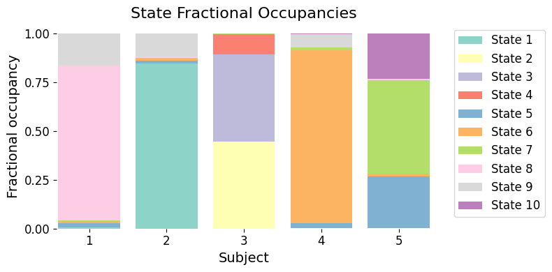
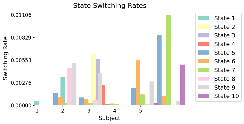

We have defined the model so that each state has a covariance (functional connectivity). We can retrieve them by using the get_covariance_matrix functions:
[17]:
graphics.plot_state_prob_and_covariance(TDE_hmm.Pi,TDE_hmm.P, TDE_hmm.get_means(),TDE_hmm.get_covariance_matrices())

Spectral analysis
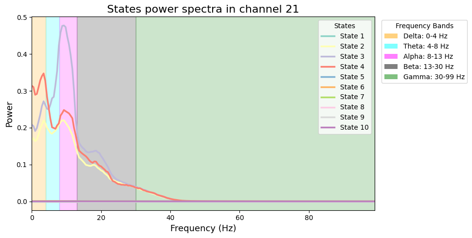
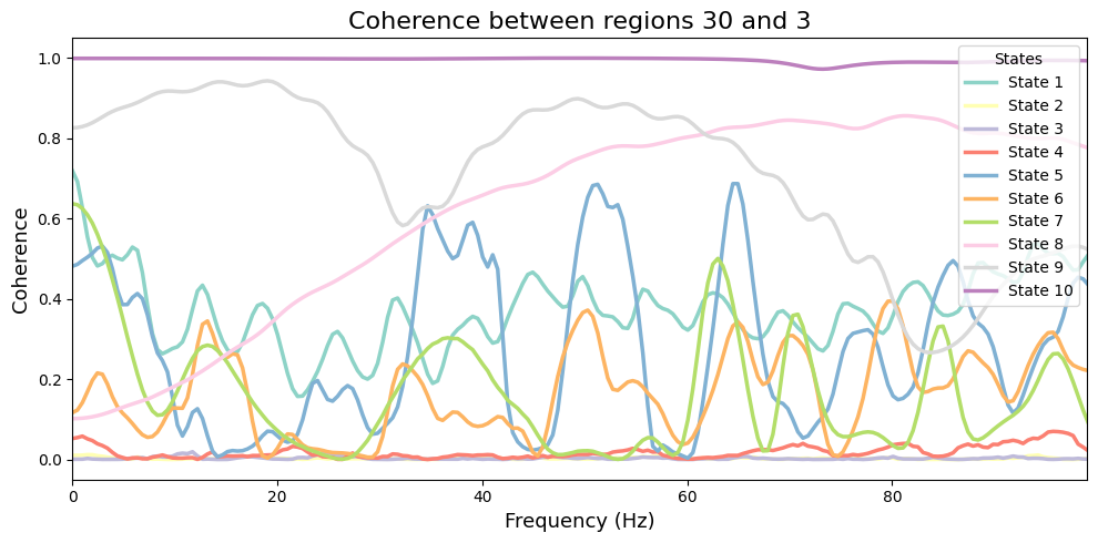
We will now use the spectral package to compute the states power spectra and coherence, and plot them.
This is done with the function spectral.multitaper_spectral_analysis that computes the states spectra using the non parametric multitaper approach. The function outputs a dictionary with the states power spectrum, states cross-channel coherence and cross-channel spectra.
The function needs as compulsory input the sampling frequency Fs of the data, which in our case is 250Hz, so we will specify Fs=250. The function also needs the Gamma (i.e., the state probability time courses) to compute the power spectrum of each state. We can input the padded Gamma, or the original gamma, specifying in the options the embeddedlags used to train the HMM. In this last case, the function will pad the Gamma first.
Other possible options for the spectral analysis are:
fpass, the frequency range for the power spectrum estimation.win, the length of the window used to compute the power spectrumn_tapers, the number of multitapers to usetapers_res, the resolution of the multitapers
[18]:
# get states spectral properties
options_tde = {'embeddedlags':list(lags), 'fpass':[0,100], 'win':1500,'n_tapers':9,'tapers_res':5}
spectral_measures = spectral.multitaper_spectral_analysis(X_preproc, idx_data, Fs=250, Gamma=stc_tde, options=options_tde)
/Users/au673157/anaconda3/lib/python3.11/site-packages/glhmm/spectral.py:303: ComplexWarning: Casting complex values to real discards the imaginary part
  psdc[j,:,:,:,k] = psdc_sk.transpose(2,0,1)
[19]:
# plot the state power spectra for a specific session, and channel
selected_channel = 21
selected_session = 2

f = spectral_measures['f']
psd = spectral_measures['p']

graphics.plot_state_psd(psd[selected_session,:,selected_channel],
                        f,
                        highlight_freq=True,
                        title="States power spectra in channel %d"%selected_channel)
[20]:
# for a specific session, plot the state coherence between two channels
coh = spectral_measures['coh']
chann_1 = 30
chann_2 = 3
graphics.plot_state_coherence(coh[selected_session,:,chann_1,chann_2],
                              f,
                              title='Coherence between regions %d and %d'%(chann_1,chann_2),
                              highlight_freq=False)
[ ]:
MAR-HMM Example: two-channel MEG data
For this example, we will use MEG data from subjects performing a simple motor task. The data consist of 10 minute sessions of subjects who were asked to rest and tap with their left finger once every roughly 30 seconds (but without counting the time in between taps).
Each subject session data is stored as a 2D matrix with the shape of (No. of timepoints, No. of channels). Here there are only two channels from the motor cortex.
We will use a subset of data collected and used for the original MAR-HMM paper
Load and preprocess data
Donwload the data from the OSF website and into ‘example_data’ folder. If you prefer, you can also directly download the files from the OSF project page.
[22]:
! osf -p 8qcyj fetch MEG_data/data_MEG_MAR.pkl ./example_data/data_MEG_MAR.pkl
100%|██████████████████████████████████| 15.9M/15.9M [00:00<00:00, 28.1Mbytes/s]
[23]:
# Loading the data in the notebook

with open("./example_data/data_MEG_MAR.pkl", "rb") as f:
    data_meg_mar = pickle.load(f)

# Display data information
print(f"Number of subjects in data_meg: {len(data_meg_mar)}")
Number of subjects in data_meg: 4
[24]:
# concatenate subject data
X_concat = []
for j in range(len(data_meg_mar)):
    X_concat.extend(data_meg_mar[j])

X_concat = np.array(X_concat)

# Get the start and end indices for each session
idx_data = statistics.get_indices_from_list(data_meg_mar)
[25]:
# show the indices of the subject/session dat
idx_data
[25]:
array([[     0, 300000],
       [300000, 540000],
       [540000, 762000],
       [762000, 996000]])
[26]:
# Preprocess data
X_preproc = preproc.preprocess_data(X_concat, idx_data)[0]
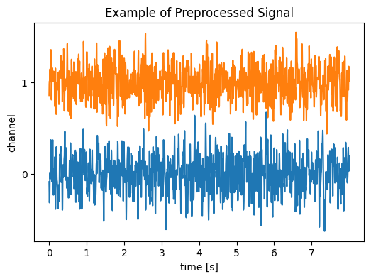
[27]:
# visualize some data
# decide on a plotting range of the signal
plot_range = np.arange(200000,202000)

Fs = 250 # sampling frequency of the signal
n_regions = X_preproc.shape[1]

# plot each parcel separately
fig = plt.figure(figsize=(6,4))
for i in range(n_regions):
    plt.plot(X_preproc[plot_range,i]+i*5)

plt.xticks(np.arange(0,len(plot_range),Fs),np.arange(int(len(plot_range)/Fs)))
plt.xlabel('time [s]')
plt.yticks(np.arange(0,n_regions*5,5),np.arange(n_regions))
plt.ylabel('channel')
plt.title('Example of Preprocessed Signal')
plt.show()
Initialise and train a MAR-HMM
We first initialise the glhmm object, which we here call MAR_hmm. By specifying the parameters of the glhmm object, we define which type of model we want to fit and how states should be defined.
In the case of the MAR-HMM, this is done with two steps: we will first construct the data to regress, and the data to predict, then we will run a decoding (i.e. Gaussian Linear) HMM on the embedded data. For more information about the decoding (Gaussian Linear) HMM, see the paper Vidaurre et al., (2025) and the notebook GLHMM_example.
For the first step, we will use the build_data_maroption in the preprocessing module. This will create an embedded version of the data X and Y, so that in the GLHMM X will be used to predict Y. To create the X and Y embeddings of the data, the function will need the order, indicating how many points back in time will be used to predict the next time point. In this specific case, we will use order=5. See original MAR-HMM paper
for more information about the model.
We will then run a GLHMM on the embedded data, to predict Y from X.
We model 4 states by setting the parameter K=3. We will also specify the covariance type as covtype='full' and no means modelling. So our states will be characterised only by functional connectivity (covariance).
[28]:
# build data MAR
autoregressive_order = 5
data = preproc.build_data_autoregressive(X_preproc,idx_data,autoregressive_order)
X_embed = data[0]
Y_embed = data[1]
idx_mar = data[2].astype(int)
[29]:
# instantiate model
MAR_hmm = glhmm.glhmm(model_beta='state', model_mean='state', K=3, covtype='full')
[30]:
# train HMM
stc_mar, xi_mar, fe_mar = MAR_hmm.train(X=X_embed,Y=Y_embed,indices=idx_mar)
Init repetition 1 free energy = -409995.47743206273
Init repetition 2 free energy = -410007.32170446805
Init repetition 3 free energy = -409711.58471609437
Init repetition 4 free energy = -416096.45643933036
Init repetition 5 free energy = -410827.13787181646
Best repetition: 4
Cycle 1 free energy = -380134.8511688909
Cycle 2 free energy = -393346.9872322161
Cycle 3, free energy = -399627.6069583118, relative change = 0.3222027605508867
Cycle 4, free energy = -404563.0874407205, relative change = 0.20203998469182397
Cycle 5, free energy = -408425.376168671, relative change = 0.13652234194948656
Cycle 6, free energy = -411402.4979490233, relative change = 0.0952141298412003
Cycle 7, free energy = -413658.15037918993, relative change = 0.06728611095275565
Cycle 8, free energy = -415350.6004637728, relative change = 0.04805946539461588
Cycle 9, free energy = -416626.60474234546, relative change = 0.03496692138962858
Cycle 10, free energy = -417608.86580660404, relative change = 0.026211791657626392
Cycle 11, free energy = -418390.67667228915, relative change = 0.020436387279518065
Cycle 12, free energy = -419037.87645436387, relative change = 0.016636232717777737
Cycle 13, free energy = -419594.2261453409, relative change = 0.01409930317723119
Cycle 14, free energy = -420087.07303765486, relative change = 0.012335906972405414
Cycle 15, free energy = -420532.0372806496, relative change = 0.011014733594655202
Cycle 16, free energy = -420936.5265899372, relative change = 0.009913546566741871
Cycle 17, free energy = -421302.47081316076, relative change = 0.00888912758098903
Cycle 18, free energy = -421628.84463883407, relative change = 0.007865567962498451
Cycle 19, free energy = -421913.89975651563, relative change = 0.0068229202750682005
Cycle 20, free energy = -422156.7194454287, relative change = 0.005778412499775442
Cycle 21, free energy = -422358.25342684373, relative change = 0.004773039846098059
Cycle 22, free energy = -422521.829866545, relative change = 0.0038591200582622958
Cycle 23, free energy = -422652.6460666326, relative change = 0.003076739995623617
Cycle 24, free energy = -422756.66690690524, relative change = 0.002440553938669501
Cycle 25, free energy = -422839.6758782313, relative change = 0.001943784382468087
Cycle 26, free energy = -422906.6974947578, relative change = 0.0015669563575981935
Cycle 27, free energy = -422961.7530572823, relative change = 0.001285536896130175
Cycle 28, free energy = -423007.868895087, relative change = 0.0010756377845664122
Cycle 29, free energy = -423047.2342537378, relative change = 0.0009173426368087528
Cycle 30, free energy = -423081.40668211365, relative change = 0.0007956966040115935
Cycle 31, free energy = -423111.4963586305, relative change = 0.0007001401897236219
Cycle 32, free energy = -423138.30439810985, relative change = 0.0006233927153819875
Cycle 33, free energy = -423162.41818304046, relative change = 0.000560426410414532
Cycle 34, free energy = -423184.2754586244, relative change = 0.0005077251541588786
Cycle 35, free energy = -423204.20778640424, relative change = 0.000462796042133579
Cycle 36, free energy = -423222.4706170679, relative change = 0.00042385332254459755
Cycle 37, free energy = -423239.2645159675, relative change = 0.00038960973124509574
Cycle 38, free energy = -423254.7503324722, relative change = 0.00035913387566010473
Cycle 39, free energy = -423269.0600942226, relative change = 0.00033174972039400546
Cycle 40, free energy = -423282.3048338777, relative change = 0.00030696457218429204
Cycle 41, free energy = -423294.5802015379, relative change = 0.0002844171623707729
Cycle 42, free energy = -423305.97046236385, relative change = 0.0002638398311739737
Cycle 43, free energy = -423316.55128324317, relative change = 0.0002450302061127081
Cycle 44, free energy = -423326.3915691258, relative change = 0.00022782900983525233
Cycle 45, free energy = -423335.55452459224, relative change = 0.0002121019972980551
Cycle 46, free energy = -423344.0980896762, relative change = 0.00019772538733660763
Cycle 47, free energy = -423352.0749239072, relative change = 0.0001845753507031368
Cycle 48, free energy = -423359.532164634, relative change = 0.0001725227475370654
Cycle 49, free energy = -423366.5112211271, relative change = 0.0001614339233032839
Cycle 50, free energy = -423373.04783657205, relative change = 0.00015117687481668726
Cycle 51, free energy = -423379.17253779, relative change = 0.00014163018458945403
Cycle 52, free energy = -423384.91143498494, relative change = 0.00013269107972708387
Cycle 53, free energy = -423390.2872076109, relative change = 0.00012427970027056227
Cycle 54, free energy = -423395.32007381, relative change = 0.00011633868810241035
Cycle 55, free energy = -423400.02858935494, relative change = 0.00010882922076539903
Cycle 56, free energy = -423404.4302096855, relative change = 0.00010172551774608645
Cycle 57, free energy = -423408.5416259779, relative change = 9.500960627460148e-05
Cycle 58, free energy = -423412.3789284274, relative change = 8.866732108242926e-05
Cycle 59, free energy = -423415.9576597834, relative change = 8.268576397803254e-05
Cycle 60, free energy = -423419.2928116792, relative change = 7.705197916813049e-05
Cycle 61, free energy = -423422.3987998933, relative change = 7.175246425507793e-05
Cycle 62, free energy = -423425.2894388231, relative change = 6.677315003894696e-05
Cycle 63, free energy = -423427.9779245086, relative change = 6.209959610168954e-05
Cycle 64, free energy = -423430.47682839783, relative change = 5.771723704517751e-05
Cycle 65, free energy = -423432.79810085904, relative change = 5.361160576174069e-05
Cycle 66, free energy = -423434.9530820354, relative change = 4.976850125414391e-05
Reached early convergence
Finished training in 766.37s : active states = 3
[31]:
# get vpath
vpath_mar = MAR_hmm.decode(X=X_embed, Y=Y_embed, viterbi=True)
[32]:
# save your trained hmm
hmm_dict = {'hmm':MAR_hmm,'stc':stc_mar,'xi':xi_mar,'fe':fe_mar,'vpath':vpath_mar}
with open("./example_data/hmm_mar.pkl", "wb") as fp:
    pickle.dump(hmm_dict, fp, pickle.HIGHEST_PROTOCOL)
[30]:
# or download the trained model
! osf -p 8qcyj fetch MEG_data/hmm_mar.pkl ./example_data/hmm_mar.pkl
100%|████████████████████████████████████| 120M/120M [00:03<00:00, 39.0Mbytes/s]
[31]:
# and load it into your notebook
# load into the notebook
with open('./example_data/hmm_mar.pkl', "rb") as f:
    hmm_dict = pickle.load(f)

MAR_hmm = hmm_dict['hmm']
stc_mar = hmm_dict['stc']
vpath_mar = hmm_dict['vpath']
[33]:
# Pad Gamma
T = auxiliary.get_T(idx_data)
options_mar ={'order':autoregressive_order}
paddedGamma = auxiliary.padGamma(stc_mar, T, options_mar)
paddedVP = auxiliary.padGamma(vpath_mar, T, options_mar)

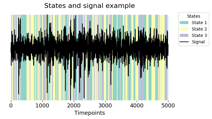
# plot state time courses with signal
plotting_range = np.arange(5000,10000)
graphics.plot_vpath(paddedVP[plotting_range], signal=X_preproc[plotting_range,1].copy(), title="States and signal example")
[34]:
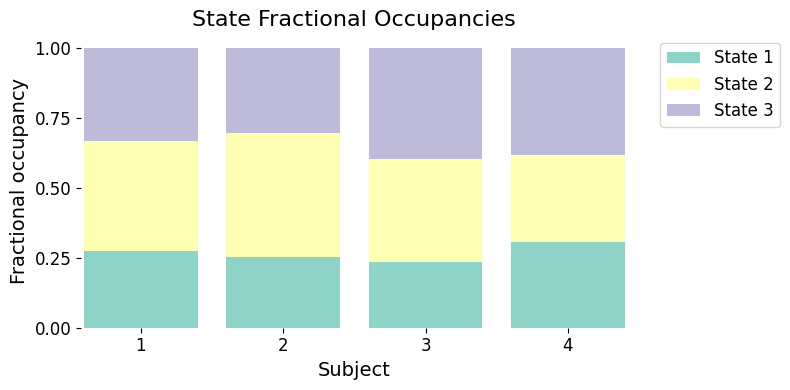
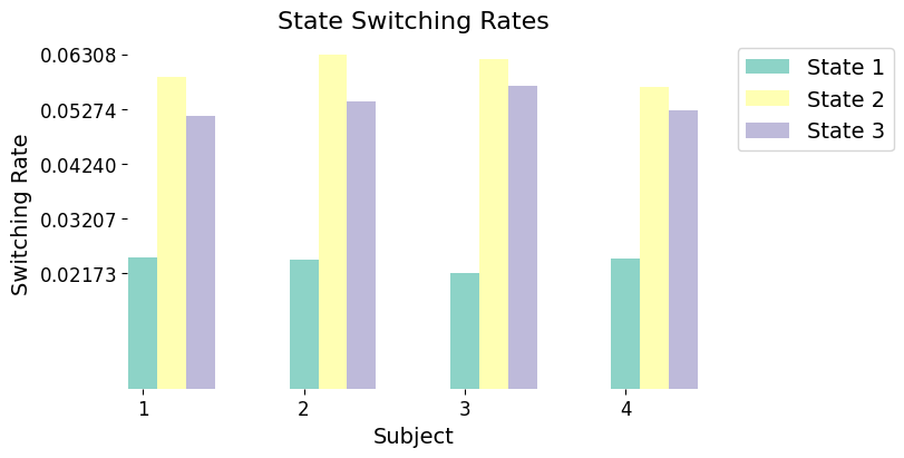
# inspect states metrics
FO = utils.get_FO(stc_mar, indices=idx_mar)
SR = utils.get_switching_rate(stc_mar, indices=idx_mar)
LTmean, LTmed, LTmax = utils.get_life_times(vpath_mar, indices=idx_mar)

# plot some relevant statistics
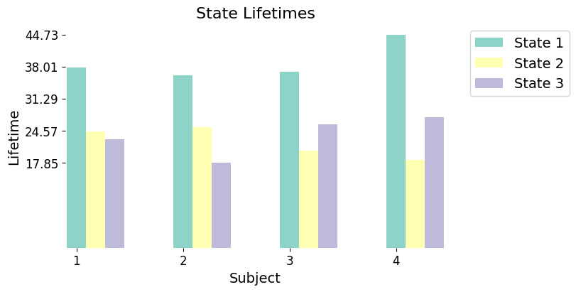
graphics.plot_FO(FO)
graphics.plot_switching_rates(SR)
graphics.plot_state_lifetimes(LTmean)
[35]:
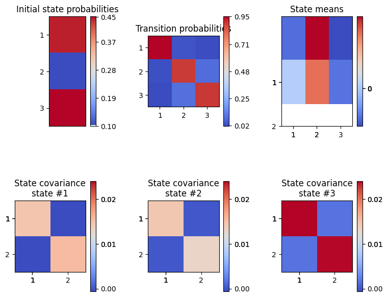
# plot the states covariance matrices
graphics.plot_state_prob_and_covariance(MAR_hmm.Pi,MAR_hmm.P, MAR_hmm.get_means(),MAR_hmm.get_covariance_matrices())
Relate behavioural outcome to states probability
As mentioned, these data were recorded while subjects would rest and tap their left finger occasionally. We will now take the timings of the tappings and align the state time courses to them, to explore the relation between the states and correlates of movement in the data.
We will download the tapping onset from the OSF folder first.
This is stored as a boolean vector (indicating the exact tap timing) of shape (No. of timepoints).
[36]:
# download onset
! osf -p 8qcyj fetch MEG_data/onset_tap_MAR.pkl ./example_data/onset_tap_MAR.pkl
100%|████████████████████████████████████| 996k/996k [00:00<00:00, 11.1Mbytes/s]
[37]:
# load the onset data into the notebook
with open('./example_data/onset_tap_MAR.pkl', "rb") as f:
    onset = pickle.load(f)
[38]:
# concatenate the onset
onset_concat = []

for i in range(len(onset)):
    onset_concat.extend(onset[i])

onset_concat = np.array(onset_concat)


# find the exact timing of the onset
onset_timing = np.where(onset_concat)[0]
[39]:
# now select a window around the timings - let's say 4 seconds, from -2 to +2 after the tapping

state_around_tap = []
for i in onset_timing:
    state_around_tap.append(paddedGamma[i-500:i+501,:])

state_around_tap = np.array(state_around_tap)
[40]:
# plot average state probability around finger tapping
K=3
cmap = plt.get_cmap('Set3')
component_colors = [cmap(i) for i in range(K)]
plt.figure()
for k in range(K):
    plt.plot(np.arange(-500,501),np.mean(state_around_tap[:,:,k],0), color=component_colors[k], label='state %d'%(k+1))
plt.xticks(np.arange(-500,501,Fs), np.arange(-2,3))
plt.vlines(x=0, ymin=0.15,ymax=0.65,linestyle='--', color='k', label='tap')
#plt.yticks([0,0.5,1])
plt.legend()
plt.xlabel('Time [s]')
plt.ylabel('Probability')
plt.title('States probability around finger tapping onset')
plt.show()

Get states spectral properties
[41]:
# get states spectral properties
#options = {'order':autoregressive_order}
spectral_measures = spectral.multitaper_spectral_analysis(X_preproc, idx_data, Fs=250, Gamma=paddedGamma, options={'fpass':[0,50]})
[42]:
# plot state power spectra per channel
select_subject = 2
cmap = plt.get_cmap('Set3')
component_colors = [cmap(i) for i in range(K)]
f = spectral_measures['f']
psd = spectral_measures['p']
fig, axs= plt.subplots(ncols=2, figsize=(10,4))
for i in range(2):
    for k in range(K):
        axs[i].plot(f,psd[select_subject,:,i,k], color=component_colors[k],label='state %d'%(k+1))
        axs[i].set_xlabel('frequency (Hz)')
        axs[i].set_ylabel('power (a.u.)')
        axs[i].legend()
        axs[i].set_title("channel %d"%(i+1))
fig.suptitle('states power spectra')
plt.show()

[45]:
# for a specific session, plot the state coherence between two channels
K=3
coh = spectral_measures['coh']
chann_1 = 0
chann_2 = 1
fig = plt.figure()
for k in range(K):
    plt.plot(f,coh[select_subject,:,chann_1,chann_2,k],color=component_colors[k], label='state %d'%(k+1))
    plt.xlabel('frequency (Hz)')
    plt.ylabel('power (a.u.)')
    plt.legend()
    plt.title("cross-channel coherence between ch %d and %d"%(chann_1,chann_2))
plt.show()

[ ]: