Across-Sessions Within Subject Testing with GLHMM toolbox

In this tutorial, we explore how to implement the Across-sessions-test-within subjects using the GLHMM toolbox, part of the paper The Gaussian-Linear Hidden Markov Model: a Python Package. This test is ideal for studying variability across different sessions, making it particularly suited for longitudinal studies involving multiple scanning sessions.

In real-world applications, one would typically fit a Hidden Markov Model (HMM) to actual data. However, for demonstration purposes, we use synthetic data for both the brain data (\(D\)) and the behavioural variable (\(R\)) in the across_sessions_within_subject test.

The synthetic data is generated using the toolbox Genephys, developed by Vidaurre in 2023. Genephys enables the simulation of electrophysiological data in psychometric experiments, creating scenarios where a subject is exposed to various stimuli while EEG or MEG data is recorded.

For this tutorial:

• The simulated brain data (\(D\)) consists of EEG or MEG recordings with 16 channels, measured across multiple trials and sessions. Each trial consists of 250 timepoints.

• The behavioural data (\(R\)) is continuous and represents reaction times for individual trials.

While data preparation requires some explanation, running the across_sessions_within_subject test is straightforward. Simply provide the input variables (\(D\) and \(R\)) and specify the method for the analysis.

Note: Due to rendering issues when viewing this notebook through github, internal links, like the table of contents, may not work correctly. To ensure that the notebook renders correctly, you can view it through this link.

Authors: Nick Yao Larsen nylarsen@cfin.au.dk

Table of Contents

1. Load and prepare data

   • Look at data

   • Prepare data for HMM

2. Load data or initialise and train HMM

   • Data restructuring

3. Across-sessions within subject testing

   • Across-sessions within subject testing - Multivariate

   • Across-sessions within subject testing - Univariate

   • Across-trials - Multivariate

Install necessary packages

If you dont have the GLHMM-package installed, then run the following command in your terminal:

pip install git+https://github.com/vidaurre/glhmm

Import libraries

Let’s start by importing the required libraries and modules.

import numpy as np
from pathlib import Path
from glhmm import glhmm, graphics, statistics,preproc

1. Load and prepare data

First, we’ll load the synthetic data from this folder and use the glhmm toolbox to train a classic HMM on the synthetic data that represents EEG or MEG measurements.

Let’s start by loading the essential data for this tutorial:

# Get the current directory
PATH_PARENT = Path.cwd()
# Path of the location of the data
PATH_DATA = PATH_PARENT / "data_statistical_testing"

# Load D data
D_sessions = np.load(PATH_DATA/"D_sessions.npy")
# Load R data
R_sessions = np.load(PATH_DATA/"R_sessions.npy")
# Load indices
idx_sessions = np.load(PATH_DATA/"idx_sessions.npy")

print(f"Data dimension of D-session data: {D_sessions.shape}")
print(f"Data dimension of R-session data: {R_sessions.shape}")
print(f"Data dimension of indices: {idx_sessions.shape}")

Data dimension of D-session data: (250, 1500, 16)
Data dimension of R-session data: (1500,)
Data dimension of indices: (10, 2)

Look at data

Now we can look at the data structure.

• D_sessions: 3D array of shape (n_timepoints, n_trials, n_features)

• R_sessions: 3D array of shape (n_trials,)

• idx_sessions: 2D array of shape (n_sessions, 2)

D_sessions represents the data collected from the subject, structured as a list with three elements: [250, 1500, 16]. The first element indicates that the subject underwent measurement across 250 timepoints. The second element, 1500, corresponds to the total number of trials conducted. In this context, 10 distinct sessions were executed, each comprising 150 trials, lead up to a total of 1500 trials (150*10). Each individual trial involved the measurement of 16 channels within the EEG or MEG scanner.

R_sessions simulates the measured reaction time for each trial that the subject undergoes at different sessions.

Lastly, we have idx_sessions = [10, 2]. This indicates the number of sessions conducted, which in this case is 10. The values in each row represent the start and end indices of the trials.

Prepare data for HMM

When you’re getting into training a Hidden Markov Model (HMM), the input data needs to follow a certain setup. The data shape should look like ((number of timepoints * number of trials), number of features). This means you’ve lined up all the trials from different sessions side by side in one long row. The second dimension is the number of features, which could be the number of parcels or channels.

So, in our scenario, we’ve got this data matrix, D_session, shaped like [250, 1500, 16] (timepoints, trials, channels). Now, when we bring all those trials together, it’s like stacking them up to create a new design matrix, and it ends up with a shape of [375000, 16] (timepoints * trials, channels). Beside that we also need to update R_session and idx_sessions to sync up with the newly concatenated data. To make life easier, we’ve got the function get_concatenate_sessions. It does the heavy lifting for us.

D_con,R_con,idx_con=statistics.get_concatenate_sessions(D_sessions, R_sessions, idx_sessions)
print(f"Data dimension of the concatenated D-data: {D_con.shape}")
print(f"Data dimension of the concatenated R-data: {R_con.shape}")
print(f"Data dimension of the updated time stamp indices: {idx_con.shape}")

Data dimension of the concatenated D-data: (375000, 16)
Data dimension of the concatenated R-data: (375000,)
Data dimension of the updated time stamp indices: (10, 2)

For a quick sanity check, let’s verify whether the concatenation was performed correctly on D_sessions. We’ve essentially stacked up every timepoint from each trial sequentially.

To do this, we can compare a slice of our original design matrix, say D_sessions[:, 0, :], with the corresponding slice in the concatenated data, D_con[0:250, :].

If the comparison D_sessions[:, 0, :] == D_con[0:250, :] holds true, we’re essentially confirming that all timepoints in the first trial align perfectly with the first 250 values in our concatenated data. It’s like double-checking to make sure everything lined up as expected.

np.array_equal(D_sessions[:, 0, :], D_con[0:250, :])

True

Here, it’s evident that the concatenation process has been executed accurately.

Next up, let’s confirm if the values in idx_con have been appropriately updated. Each row in this matrix should represent the total count of timepoints and trials for each of the 10 sessions. In our case, it should total to 37500 for each session (calculated as 250 time points * 150 trials).

# Look at idx_con
idx_con

array([[     0,  37500],
       [ 37500,  75000],
       [ 75000, 112500],
       [112500, 150000],
       [150000, 187500],
       [187500, 225000],
       [225000, 262500],
       [262500, 300000],
       [300000, 337500],
       [337500, 375000]], dtype=int32)

Indeed, each session now aligns with 37500 datapoints. This means that when we pooled together the timepoints and trials, the count for each session ended up exactly as expected. It’s a reassuring confirmation that our concatenation didn’t miss a beat.

Please take note: If the measurements haven’t been continuously recorded within a single session but have been pre-processed and exported on a trial-by-trial basis, we’ll need to construct the indices in a different manner. In our case, where we have 250 timepoints for each trial, where each trial consists of 250 timepoints and there are a total of 1500 trials, the indices must be created by specifying the start and end timepoints for each trial.

You can create these indices using the get_timestamp_indices function. The following example will guide you through the process.

idx_trials =statistics.get_indices_timestamp(D_sessions.shape[0], D_sessions.shape[1])
print(f"Values in index:\n{idx_trials}\n")
print(f"Shape of index: {idx_trials.shape}")

Values in index:
[[     0    250]
 [   250    500]
 [   500    750]
 ...
 [374250 374500]
 [374500 374750]
 [374750 375000]]

Shape of index: (1500, 2)

NOTE: It is important to standardise your timeseries and, if necessary, apply other kinds of preprocessing before fitting the model.

This will be done separately for each session/subject as specified in the indices. The data provided here are already close to standardised (so the code below will not do much).

D_con_preproc,_ = preproc.preprocess_data(D_con,
                                          idx_trials)

2. Load data or initialise and train HMM

You can either load the Gamma values from a pretrained model or train your own model. If you prefer the former option, load the Gamma_sessions from the data_statistical_testing folder. The GLHMM model in question has been trained utilizing a Gaussian observation model, incorporating mean and covariance parameters for 6 distinct states.

However, if you would rather train your own model, you can use the variables D_con and idx_con as inputs and and complete this section.

Our modeling approach involves representing states as Gaussian distributions with mean and a full covariance matrix. This means that each state is characterized by a mean amplitude and a functional connectivity pattern. To specify this configuration, set covtype='full' and the number of states to K=6. If you prefer not to model the mean, you can include model_mean='no'. Optionally, you can check the hyperparameters to make sure that they correspond to how you want the model to be set up.

# Create an instance of the glhmm class
K = 6 # number of states
hmm = glhmm.glhmm(model_beta='no', K=K, covtype='full')
print(hmm.hyperparameters)

{'K': 6, 'covtype': 'full', 'model_mean': 'state', 'model_beta': 'no', 'dirichlet_diag': 10, 'connectivity': None, 'Pstructure': array([[ True,  True,  True,  True,  True,  True],
       [ True,  True,  True,  True,  True,  True],
       [ True,  True,  True,  True,  True,  True],
       [ True,  True,  True,  True,  True,  True],
       [ True,  True,  True,  True,  True,  True],
       [ True,  True,  True,  True,  True,  True]]), 'Pistructure': array([ True,  True,  True,  True,  True,  True])}

Train an HMM

Now, let’s proceed to train the HMM using the loaded data (D_con) and time indices (idx_con).

Since in this case, we are not modeling an interaction between two sets of timeseries but opting for a “classic” HMM, we set X=None. For training, Y should represent the timeseries from which we aim to estimate states (D_con), and indices should encompass the beginning and end indices of each subject (idx_con).

If you want to use the same Gamma values as used in this tutorial without training the HMM, you can just load Gamma using the code below:

# Get the current directory
PATH_PARENT = Path.cwd()
# Path of the location of the data
PATH_DATA = PATH_PARENT / "data_statistical_testing"
# Load Gamma data
Gamma = np.load(PATH_DATA/"Gamma_sessions.npy")
print(f"Data dimension of Gamma: {Gamma.shape}")

Gamma,Xi,FE = hmm.train(X=None,
                        Y=D_con_preproc.astype(np.float64),
                        indices=idx_trials)

Init repetition 1 free energy = 10424285.62136018
Init repetition 2 free energy = 10424471.457711864
Init repetition 3 free energy = 10418736.098348387
Init repetition 4 free energy = 10416991.333350975
Init repetition 5 free energy = 10413512.681879953
Best repetition: 5
Cycle 1 free energy = 10415552.22543761
Cycle 2 free energy = 10404433.474428767
Cycle 3, free energy = 10399962.798963035, relative change = 0.286776134646397
Cycle 4, free energy = 10396844.666747313, relative change = 0.16667766582172433
Cycle 5, free energy = 10394446.060602685, relative change = 0.11364481247008078
Cycle 6, free energy = 10392542.188508492, relative change = 0.08274094040171934
Cycle 7, free energy = 10390976.895951219, relative change = 0.06369365497784654
Cycle 8, free energy = 10389665.812333891, relative change = 0.05064755831851465
Cycle 9, free energy = 10388570.153590763, relative change = 0.04060691667219894
Cycle 10, free energy = 10387666.949602965, relative change = 0.03238999653987988
Cycle 11, free energy = 10386921.924499355, relative change = 0.02602225890732946
Cycle 12, free energy = 10386287.517006794, relative change = 0.021678244089158263
Cycle 13, free energy = 10385716.909915598, relative change = 0.01912522395732363
Cycle 14, free energy = 10385170.102370033, relative change = 0.01799767397258085
Cycle 15, free energy = 10384610.16658393, relative change = 0.018096267890629736
Cycle 16, free energy = 10383997.916000562, relative change = 0.019403073440377155
Cycle 17, free energy = 10383301.107497333, relative change = 0.021605716258255983
Cycle 18, free energy = 10382516.406493783, relative change = 0.02375303620848365
Cycle 19, free energy = 10381697.433626954, relative change = 0.02419075182650241
Cycle 20, free energy = 10380950.45768706, relative change = 0.021587797053583206
Cycle 21, free energy = 10380330.81922069, relative change = 0.017592666872900235
Cycle 22, free energy = 10379827.818128241, relative change = 0.01408004023951785
Cycle 23, free energy = 10379410.626232367, relative change = 0.011543260537671558
Cycle 24, free energy = 10379052.20066883, relative change = 0.009819871789324648
Cycle 25, free energy = 10378733.882826217, relative change = 0.008645632041986765
Cycle 26, free energy = 10378445.424423078, relative change = 0.007773734066309854
Cycle 27, free energy = 10378182.209982885, relative change = 0.007043466185127063
Cycle 28, free energy = 10377942.33251607, relative change = 0.006378041737981543
Cycle 29, free energy = 10377725.46424632, relative change = 0.005733196893441284
Cycle 30, free energy = 10377531.738014368, relative change = 0.0050953116354012255
Cycle 31, free energy = 10377360.167969914, relative change = 0.004492296457170692
Cycle 32, free energy = 10377208.16697361, relative change = 0.003964134272520598
Cycle 33, free energy = 10377071.903067501, relative change = 0.003541132134954935
Cycle 34, free energy = 10376946.791559195, relative change = 0.0032407745681643577
Cycle 35, free energy = 10376827.877472263, relative change = 0.003070783452279929
Cycle 36, free energy = 10376710.105669716, relative change = 0.003032064244954175
Cycle 37, free energy = 10376588.488315739, relative change = 0.0031212959269600053
Cycle 38, free energy = 10376458.11672618, relative change = 0.00333481421767484
Cycle 39, free energy = 10376314.160302727, relative change = 0.0036687951599837765
Cycle 40, free energy = 10376152.449988794, relative change = 0.004104346080424937
Cycle 41, free energy = 10375971.758992493, relative change = 0.004565155808635596
Cycle 42, free energy = 10375773.913474215, relative change = 0.004973703219483623
Cycle 43, free energy = 10375561.531036953, relative change = 0.005310796435162553
Cycle 44, free energy = 10375337.870999215, relative change = 0.005561696584734983
Cycle 45, free energy = 10375105.199401585, relative change = 0.005752501986735857
Cycle 46, free energy = 10374863.256759092, relative change = 0.00594614831368073
Cycle 47, free energy = 10374610.54661305, relative change = 0.00617244219819337
Cycle 48, free energy = 10374345.637196878, relative change = 0.006428812175010359
Cycle 49, free energy = 10374067.315469444, relative change = 0.006708987138883736
Cycle 50, free energy = 10373776.412767604, relative change = 0.006963424126244926
Cycle 51, free energy = 10373480.627518022, relative change = 0.0070305209264194205
Cycle 52, free energy = 10373194.864750018, relative change = 0.006746472475274071
Cycle 53, free energy = 10372935.29376709, relative change = 0.006090794732343945
Cycle 54, free energy = 10372715.589104671, relative change = 0.005128896225937276
Cycle 55, free energy = 10372541.971970867, relative change = 0.0040366452138654784
Cycle 56, free energy = 10372412.027299708, relative change = 0.003012148222968975
Cycle 57, free energy = 10372318.436656721, relative change = 0.0021647569094890616
Cycle 58, free energy = 10372252.779479427, relative change = 0.0015163514414730298
Cycle 59, free energy = 10372207.41145504, relative change = 0.0010466771043177278
Cycle 60, free energy = 10372176.202932924, relative change = 0.0007194878717474443
Cycle 61, free energy = 10372154.638114437, relative change = 0.000496912842780475
Cycle 62, free energy = 10372139.568216968, relative change = 0.00034713142281389645
Cycle 63, free energy = 10372128.866829285, relative change = 0.0002464431132436224
Cycle 64, free energy = 10372121.120897517, relative change = 0.0001783498681604869
Cycle 65, free energy = 10372115.396574657, relative change = 0.0001317850084604177
Cycle 66, free energy = 10372111.075665914, relative change = 9.94658006658798e-05
Cycle 67, free energy = 10372107.746128097, relative change = 7.663891636552954e-05
Cycle 68, free energy = 10372105.130371124, relative change = 6.0205566554482105e-05
Cycle 69, free energy = 10372103.038814038, relative change = 4.813800321820953e-05
Cycle 70, free energy = 10372101.339909043, relative change = 3.909943316939458e-05
Cycle 71, free energy = 10372099.940770814, relative change = 3.219941689365205e-05
Cycle 72, free energy = 10372098.774599282, relative change = 2.683725940347362e-05
Cycle 73, free energy = 10372097.792451281, relative change = 2.2601790737425705e-05
Cycle 74, free energy = 10372096.957804253, relative change = 1.9207039174578052e-05
Cycle 75, free energy = 10372096.242921904, relative change = 1.645072342656288e-05
Reached early convergence
Finished training in 496.58s : active states = 6

As you can see, the datapoints in Gamma correspond to the concatenated data (375000), and the number of columns represent the six different states.

Gamma.shape

(375000, 6)

Data restructuring

Now we have trained our HMM and got our Gamma values we need to restructure the data back to the original data structure. In this case we are not doing HMM-aggregated statistics, but we will instead perform the statistical testing per time point. We will acheive this by applying the function reconstruct_concatenated_to_3D. It takes a concatenated 2D matrix and converts it into a 3D matrix. So, it will convert Gamma, shaped like [375000, 6] back to the original format for number of time points and trials shaped like [250, 1500, 6] (timepoints, trials, channels).

# Reconstruct the Gamma matrix
n_timepoints, n_trials, n_channels = D_sessions.shape[0],D_sessions.shape[1],Gamma.shape[1]
Gamma_epoch = statistics.reconstruct_concatenated_to_3D(Gamma,
                                                       n_timepoints=n_timepoints,
                                                       n_entities=n_trials,
                                                       n_features=n_channels)

As a sanity check we will see if gamma_epoch is actually structured correctly by comparing it with Gamma.

To do this, we can compare a slice of our 3D-matrix, like gamma_epoch[:, 0, :], with the corresponding slice in the concatenated 2D-data, Gamma[0:250, :].

If the comparison gamma_epoch[:, 0, :] == Gamma[0:250, :] holds true, we’re essentially confirming that all timepoints in the first trial align perfectly with the first 250 values in our concatenated data.

np.array_equal(Gamma_epoch[:, 0, :], Gamma[0:250, :])

True

3. Across-sessions within subject testing

As we move on to the next part of this tutorial, let’s dive into how we can use the test_across_sessions_within_subject function. This function helps us to find connections between HMM state occurrences (D) and behavioral variables or individual traits (R) using permutation testing.

Permutation testing

Permutation testing does not assume any particular data distribution and the procedure shuffles the data around to create a null distribution. This null distribution comes in handy for testing our hypotheses without making any assumptions about the data. This null distribution becomes our benchmark to test the question: is there any real difference or relationship between the variables we’re interested in?

Figure 5C in Vidaurre et al. 2023: A 9 x 4 matrix representing permutation testing across sessions. Each number corresponds to a trial within a session and permutations are performed between sessions, with each session containing the same number of trials.

Hypothesis

• Null Hypothesis (H0): No significant relationship exists between the independent variables and the dependent variable.

• Alternative Hypothesis (H1):: There is a significant relationship between the independent variables and the dependent variable.

Across-sessions within subject testing - Multivariate

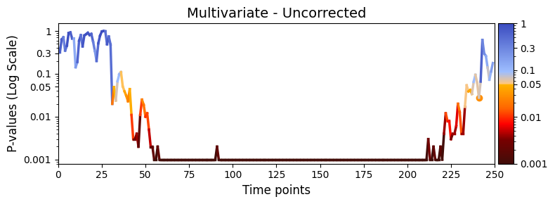
The multivariate analysis aims to evaluate whether the state time courses of our brain data (\(D\)) contribute to explaining the observed variability in behavioral measurements (\(R\)) like reaction time. By quantifying explained variance, this analysis determines whether state time courses significantly influence changes in behavioral responses.

If there is no difference in brain activity between sessions, it suggests that the brain’s response to the stimuli is consistent over time. However, if we detect differences, this could indicate that the subject’s perception of the task changes over time, as reflected by variations in brain activity across sessions.

To run the test_across_sessions_within_subject test, we set the following parameters:

Inputs:

• D_data: The state time courses of the brain data (Gamma_epoch).

• R_data: The behavioral measurements (R_trials).

• idx_data : Indices for the first and last trial for a given session (idx_trials_session)

Settings:

• method = "multivariate": Specifies that the test should perform multivariate analysis.

• Nnull_samples: Number of permutations (optional, default is 1000).

• test_statistics_option = True: Ensures the permutation distribution is exported.

Additional settings allow for the inclusion of confounding variables, which can be regressed out during the permutation testing process. For details on these settings, refer to the function documentation.

# Set the parameters for across sessions within subject testing
method = "multivariate"
Nnull_samples = 1000 # Number of permutations (default = 0)

# Perform across-subject testing
result_multivariate_session  =statistics.test_across_sessions_within_subject(D_data=Gamma_epoch,
                                                                             R_data=R_sessions,
                                                                             idx_data=idx_sessions,
                                                                             method=method,
                                                                             Nnull_samples=Nnull_samples)

Total possible permutations: 3.62e+6
Running number of permutations: 1000
performing permutation testing per timepoint

100%|██████████| 250/250 [01:49<00:00,  2.28it/s]

What we can see here is that result_multivariate_session is a dictionary containing the outcomes of a statistical analysis conducted using the specified method and test_type.

Let us break it down:

• pval: This array holds the p-values resulting from the permutation test. Each value corresponds to a behavioral variable and will have shape of 1 by q, see GLHMM paper.

• base_statistics: Stores the base statistics of the tests. In this case it is the explained variance \(R^2\)

• test_statistic: Will by default always return a list of the base (unpermuted) statistics when test_statistic_option=False. This list can store the test statistics associated with the permutation test. It provides information about the permutation distribution that is used to calculate the p-values. The output will exported if we set test_statistic_option=True

• statistical_measures: A dictionary that marks the units used as test_statistics

• test_type: Indicates the type of permutation test performed. In this case, it is across_sessions_within_subject.

• method: Specifies the analytical method employed, which is 'multivariate', which means that the analysis is carried out using regression-based permutation testing.

• max_correction: Boolean value that indicates whether Max correction has been applied when performing permutation testing

• Nnull_samples: Is the number of permutations that has been performed.

• test_summary: A dictionary summarizing the test results based on the applied method.

Visualization of results

Now that we have performed our test, we can then visualize the p-value array.

We will use the function plot_heatmap from the graphics module.

Note: Elements marked in red indicate a p-value below 0.05, signifying statistical significance.

# The alpha score we set for the p-values
alpha = 0.05
# Plot p-values
graphics.plot_p_values_over_time(result_multivariate_session["pval"],
                                 title_text ="Multivariate - Uncorrected",
                                 xlabel="Time points",
                                 alpha=alpha,
                                 num_x_ticks=11)

Multiple Comparison

To take into account for type 1 error, we can apply the Benjamini/Hochberg correction.

pval_corrected, rejected_corrected =statistics.pval_correction(result_multivariate_session,
                                                               method='fdr_bh')
# Plot p-values
graphics.plot_p_values_over_time(pval_corrected,
                                 title_text ="Multivariate - Benjamini/Hochberg",
                                 xlabel="HMM States",
                                 num_x_ticks=11)

Cluster based permutation testing

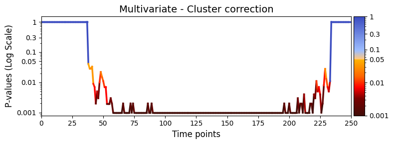
In order to provide a more strict control over Type I mistakes, we can also apply cluster-based permutation testing to control the Family-Wise Error Rate when conducting multiple comparisons. To use this p-value correction, set test_statistics_option=True while performing permutation testing, as it is an input to the function (pval_cluster_based_correction).

pval_cluster =statistics.pval_cluster_based_correction(result_multivariate_session)
# Plot p-values
graphics.plot_p_values_over_time(pval_cluster,
                                 title_text ="Multivariate - Cluster correction",
                                 xlabel="Time points",
                                 num_x_ticks=11)

Conclusion - Multivariate test

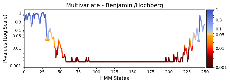
In the permutation testing across sessions, we examined the relationship between state time courses (\(D\)) and reaction time (\(R\)) across experimental sessions while preserving trial order. . Using synthetic data, the test identified significant differences from 27 to 230 timepoints. Although this extensive significance is likely due to synthetic data limitations, it highlights the toolbox’s effectiveness in detecting across-session differences. In real experiments, such periods could reflect critical cognitive or neural processes depending on the task design.

Across-sessions within subject testing - Univariate test

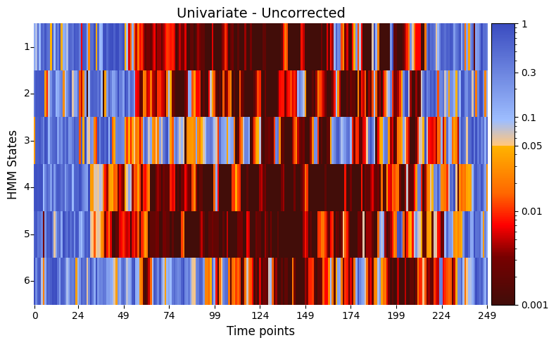
The univariate analysis examines how each state in the brain’s activity (\(D\), represented by gamma_epoch) relates to the behavioral measurements (\(R\)). This method looks for patterns between individual states and the variability in behavioral responses, such as ‘reaction time’, across sessions.

To run the test_across_sessions_within_subject test, we set the following parameters:

Inputs:

• D_data: The state time courses of the brain data (gamma_epoch).

• R_data: The behavioral measurements (R_sessions).

• idx_data : Indices for the first and last trial for a given session (idx_sessions)

Settings:

• method = "univariate": Specifies that the test should perform univariate analysis.

• Nnull_samples: Number of permutations (optional, default is 1000).

Additional settings allow for the inclusion of confounding variables, which can be regressed out during the permutation testing process. For details on these settings, refer to the function documentation.

# Set the parameters for between-subject testing
method = "univariate"
Nnull_samples = 1000 # Number of permutations (default = 1000)
# Perform across-subject testing
result_univariate =statistics.test_across_sessions_within_subject(D_data=Gamma_epoch,
                                                                  R_data=R_sessions,
                                                                  idx_data=idx_sessions,
                                                                  method=method,
                                                                  Nnull_samples=Nnull_samples)

Total possible permutations: 3.62e+6
Running number of permutations: 1000
performing permutation testing per timepoint

100%|██████████| 250/250 [07:49<00:00,  1.88s/it]

Visualization of results

Now that we have performed our test, we can then visualize the p-value matrix.

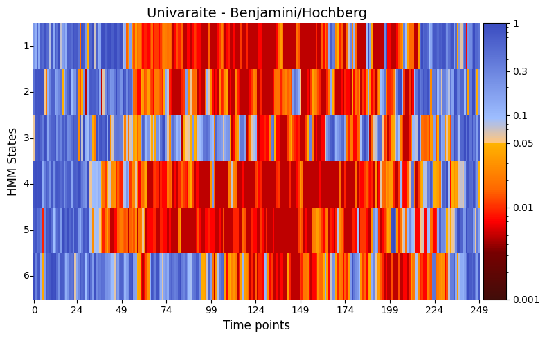
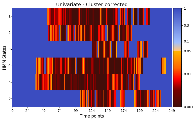
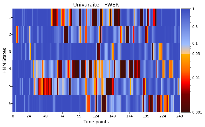
We will use the function plot_heatmap from the graphics module.

Note: Elements marked in red indicate a p-value below 0.05, signifying statistical significance.

# Plot p-values
# P-values between reaction time and each state as function of time
graphics.plot_p_value_matrix(result_univariate["pval"].T,
                             title_text ="Univariate - Uncorrected",
                             figsize=(8, 5),
                             xlabel="Time points",
                             ylabel="HMM States",
                             annot=False,
                             num_x_ticks=11)

Multiple Comparison

To be sure there is no type 1 error, we can apply the Benjamini/Hochberg to control the False Discovery Rate

alpha = 0.05 # threshold for p-values
pval_corrected, rejected_corrected =statistics.pval_correction(result_univariate,
                                                               method='fdr_bh', alpha=0.5)
# Plot p-values
graphics.plot_p_value_matrix(pval_corrected.T,
                             title_text ="Univaraite - Benjamini/Hochberg",
                             figsize=(8, 5),
                             xlabel="Time points",
                             ylabel="HMM States",
                             annot=False,
                             num_x_ticks=11)

Cluster based permutation testing

In order to provide a more strict control over Type I mistakes, we can also apply cluster-based permutation testing to control the Family-Wise Error Rate when conducting multiple comparisons.

pval_cluster =statistics.pval_cluster_based_correction(result_univariate, individual_feature=True)
# Plot p-values
graphics.plot_p_value_matrix(pval_cluster.T,
                             title_text ="Univariate - Cluster corrected",
                             figsize=(8, 5),
                             xlabel="Time points",
                             ylabel="HMM States",
                             annot=False,
                             num_x_ticks=11)

Family-Wise Error Rate (FWER) correction

Applying FWER correction

# Correct for FWER
pval_FWER = statistics.pval_FWER_correction(result_univariate)

# Correct p-values using FWER
graphics.plot_p_value_matrix(pval_FWER.T,
                             title_text ="Univaraite - FWER",figsize=(8, 5),
                             xlabel="Time points",
                             ylabel="HMM States",
                             annot=False,
                             num_x_ticks=11)

Conclusion - Univariate

Using synthetic data, the univariate test compared individual states to reaction time in a pairwise manner. After correcting p-values with the Benjamini/Hochberg method, varying degrees of significance were observed for states 1, 2, 3, 5, and 6 during the same timespan as the multivariate test (27 to 230 timepoints), while state 4 showed minimal or no significance.

When Family-Wise Error Rate (FWER) correction using the MaxT method was applied separately to the uncorrected data, it removed many of the initially significant points. This indicates that some of the findings from the Benjamini/Hochberg-corrected results may still include false positives, emphasizing the importance of choosing the appropriate correction method depending on the analysis context.

Across-trials within session testing - Multivariate

From our previous result, it is evident that there are variations at specific time windows across multiple sessions. This indicates significant changes occurring during each experimental session in which the subject is involved.

An intriguing aspect of this dataset is the opportunity to delve into trial-by-trial variability within each experimental session. Even though we observe a significant difference across sessions, it’s possible that there are specific periods across trials that shows variability. This hypothesis can be tested using the function test_across_trials_within_session.

To run the test_test_across_trials_within_session test, we set the following parameters:

Inputs:

• D_data: The state time courses of the brain data (gamma_epoch).

• R_data: The behavioral measurements (R_trials).

• idx_data : Indices for the first and last trial for a given session (idx_trials_session)

Settings:

• method = "multivariate": Specifies that the test should perform multivariate analysis.

• Nnull_samples: Number of permutations (optional, default is 1000).

Additional settings allow for the inclusion of confounding variables, which can be regressed out during the permutation testing process. For details on these settings, refer to the function documentation.

# Set the parameters for across trials testing
method = "multivariate"
Nnull_samples = 1000 # Number of permutations (default = 1000)

# Perform across-trial testing
result_multivaraite_trials  =statistics.test_across_trials(Gamma_epoch,
                                                           R_sessions,
                                                           idx_sessions,
                                                           method=method,
                                                           Nnull_samples=Nnull_samples)

performing permutation testing per timepoint
Total possible permutations: 3.70e+2627
Running number of permutations: 1000

100%|██████████| 250/250 [01:46<00:00,  2.35it/s]

Visualization of results

Now that we have performed our test, we can then visualize the p-value array.

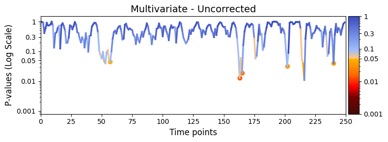
We will use the function plot_p_values_over_time from the graphics module.

Note: Elements marked in red indicate a p-value below 0.05, signifying statistical significance.

# Plot p-values
graphics.plot_p_values_over_time(result_multivaraite_trials["pval"],
                                 title_text ="Multivariate - Uncorrected",
                                 xlabel="Time points",
                                 num_x_ticks=11)

# Multiple correction
alpha = 0.05
pval_corrected, rejected_corrected =statistics.pval_correction(result_multivaraite_trials,
                                                               method='fdr_bh',alpha=alpha)
# Plot p-values
graphics.plot_p_values_over_time(pval_corrected,
                                 title_text ="Multivariate - Benjamini/Hochberg",
                                 xlabel="HMM States",
                                 num_x_ticks=11)

Cluster based permutation testing

In order to provide a more strict control over Type I mistakes, we can also apply cluster-based permutation testing to control the Family-Wise Error Rate when conducting multiple comparisons.

pval_cluster =statistics.pval_cluster_based_correction(result_multivaraite_trials)
# Plot p-values
graphics.plot_p_values_over_time(pval_cluster,
                                 title_text ="Multivariate - Cluster correction",
                                 xlabel="Time points",
                                 num_x_ticks=11)

Conclusion - Multivariate trials

In the multivariate test across trials, we examined the relationship between state time courses (\(D\)) and reaction time (\(R\)) across different trials within experimental sessions.

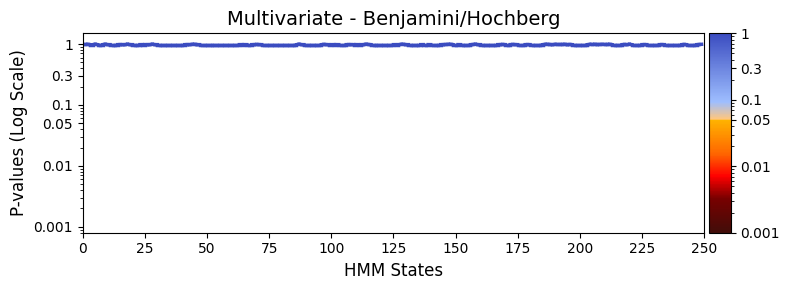
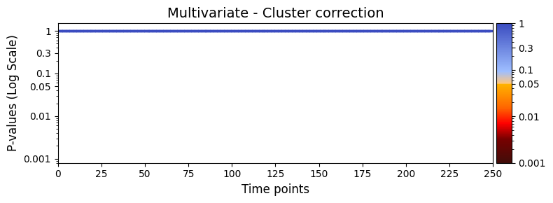
After correcting the p-values, no significant differences were found across the time points. This suggests a stable relationship between state time courses and reaction time throughout trials within each session. This stability indicates that, within a single session, the subject’s performance remains relatively consistent in terms of the observed state time courses and corresponding reaction times.

This finding is consistent with how the synthetic data was generated, where reaction times were designed to remain stable across trials within a session but to vary across sessions. While this tutorial primarily focuses on variability between sessions, incorporating trial-to-trial variability within a session provides a more comprehensive view of the data, offering finer insights into performance dynamics.